STATS19 Data exploration
A mockup guide for newcomers to STATS19
Carlos Cámara-Menoyo
This is a mock report exploring data from STATS19’s R package1 made by someone who has never worked with that kind of dataset before. STATS19 provides three types of datasets: accidents, vehicles and casualties.
Accidents 2018
Initial exploration
Let’s see how many observations do we have as well as the variables’ number and types.
| Name | accidents2018 |
| Number of rows | 122635 |
| Number of columns | 31 |
| _______________________ | |
| Column type frequency: | |
| Date | 1 |
| factor | 22 |
| numeric | 8 |
| ________________________ | |
| Group variables | None |
Variable type: Date
| skim_variable | n_missing | complete_rate | min | max | median | n_unique |
|---|---|---|---|---|---|---|
| datetime | 13 | 1 | 2018-01-01 | 2018-12-31 | 2018-07-05 | 365 |
Variable type: factor
| skim_variable | n_missing | complete_rate | ordered | n_unique | top_counts |
|---|---|---|---|---|---|
| accident_index | 0 | 1.00 | FALSE | 122635 | 201: 1, 201: 1, 201: 1, 201: 1 |
| police_force | 0 | 1.00 | FALSE | 51 | Met: 25390, Wes: 5490, Ken: 4403, Wes: 4132 |
| accident_severity | 0 | 1.00 | FALSE | 3 | Sli: 97799, Ser: 23165, Fat: 1671 |
| date | 0 | 1.00 | FALSE | 365 | 201: 504, 201: 498, 201: 491, 201: 488 |
| day_of_week | 0 | 1.00 | FALSE | 7 | Fri: 20021, Thu: 18656, Wed: 18397, Tue: 17950 |
| time | 13 | 1.00 | FALSE | 1438 | 17:: 1154, 18:: 1093, 17:: 1086, 16:: 1069 |
| local_authority_district | 0 | 1.00 | FALSE | 380 | Bir: 2614, Lee: 1548, Wes: 1509, Lam: 1287 |
| local_authority_highway | 0 | 1.00 | FALSE | 207 | Ken: 3811, Sur: 3113, Lan: 2676, Ham: 2615 |
| first_road_class | 0 | 1.00 | FALSE | 6 | A: 53499, Unc: 43355, B: 14210, C: 7005 |
| road_type | 0 | 1.00 | FALSE | 6 | Sin: 88323, Dua: 19473, Rou: 7573, One: 3366 |
| junction_detail | 0 | 1.00 | FALSE | 10 | Not: 52076, T o: 35958, Cro: 11422, Rou: 9974 |
| junction_control | 0 | 1.00 | FALSE | 5 | Dat: 54842, Giv: 53259, Aut: 13323, Sto: 750 |
| second_road_class | 52211 | 0.57 | FALSE | 6 | Unc: 48631, A: 12213, B: 4662, C: 4168 |
| pedestrian_crossing_human_control | 0 | 1.00 | FALSE | 4 | Non: 117924, Dat: 3173, Con: 1116, Con: 422 |
| pedestrian_crossing_physical_facilities | 0 | 1.00 | FALSE | 7 | No : 94877, Ped: 9753, Pel: 7169, Zeb: 4583 |
| light_conditions | 0 | 1.00 | FALSE | 5 | Day: 88435, Dar: 24746, Dar: 6120, Dar: 2477 |
| weather_conditions | 0 | 1.00 | FALSE | 10 | Fin: 99221, Rai: 12789, Unk: 3666, Oth: 2603 |
| road_surface_conditions | 0 | 1.00 | FALSE | 6 | Dry: 90546, Wet: 28215, Fro: 1417, Dat: 1223 |
| special_conditions_at_site | 0 | 1.00 | FALSE | 9 | Non: 118495, Dat: 1524, Roa: 1372, Aut: 284 |
| carriageway_hazards | 0 | 1.00 | FALSE | 7 | Non: 119170, Dat: 1325, Oth: 1072, Any: 376 |
| urban_or_rural_area | 1 | 1.00 | FALSE | 3 | Urb: 82583, Rur: 39996, Una: 55 |
| lsoa_of_accident_location | 6445 | 0.95 | FALSE | 27965 | E01: 165, E01: 123, E01: 84, E01: 82 |
Variable type: numeric
| skim_variable | n_missing | complete_rate | mean | sd | p0 | p25 | p50 | p75 | p100 | hist |
|---|---|---|---|---|---|---|---|---|---|---|
| longitude | 55 | 1 | -1.26 | 1.40 | -7.27 | -2.19 | -1.15 | -0.14 | 1.76 | ▁▁▅▇▃ |
| latitude | 55 | 1 | 52.43 | 1.38 | 49.91 | 51.47 | 51.89 | 53.39 | 60.76 | ▇▆▁▁▁ |
| number_of_vehicles | 0 | 1 | 1.85 | 0.72 | 1.00 | 1.00 | 2.00 | 2.00 | 24.00 | ▇▁▁▁▁ |
| number_of_casualties | 0 | 1 | 1.31 | 0.76 | 1.00 | 1.00 | 1.00 | 1.00 | 59.00 | ▇▁▁▁▁ |
| first_road_number | 0 | 1 | 836.74 | 1670.33 | 0.00 | 0.00 | 41.00 | 580.00 | 9621.00 | ▇▁▁▁▁ |
| speed_limit | 0 | 1 | 37.11 | 14.07 | 20.00 | 30.00 | 30.00 | 40.00 | 70.00 | ▇▁▁▂▁ |
| second_road_number | 0 | 1 | 291.80 | 1129.17 | -1.00 | 0.00 | 0.00 | 0.00 | 9620.00 | ▇▁▁▁▁ |
| did_police_officer_attend_scene_of_accident | 0 | 1 | 1.29 | 0.47 | -1.00 | 1.00 | 1.00 | 2.00 | 3.00 | ▁▁▇▃▁ |
The table above shows that overall we do not have significant missing data in any of the 16 variables as well as some basic statistics of the (few) numerical variables. Now let’s see the mode for every variable.
The tables above pose interesting (basic) research questions to be explored. As an example, seeing that the day of the week were most accidents take place is Friday, I would like to know if most accidents happen during weekdays or weekend. We could use that data as a proxy to infer if professional drivers are more or less involved in accidents than amateurs, especially if we combine that with the hour of the day.
Surprisingly, most accidents take place on dry conditions with sunny days and good visibility, so, apparently, weather does not have such as big impact as I might have guessed on the first sight, although verifying it would require further analysis.
Accidents’ evolution over time
There have been a total of 122,635 accidents in 2018, out of which a 1% were fatal, 19% were serious, and 80% were slight. However, let’s see how these figures have been evolved through time and if there has been an increase or decrease on the number of accidents.
Wile the number of accidents in UK is high, we can see an overall tendency in number of accidents to decrease over time, but can we observe other patterns?
| year | Fatal | Fatal variation | Serious | Serious variation | Slight | Slight variation | Total | Total variation |
|---|---|---|---|---|---|---|---|---|
| 2009 | 2057 | NA | 21997 | NA | 139500 | NA | 163554 | NA |
| 2010 | 1731 | -18.83% | 20440 | -7.62% | 132243 | -5.4876% | 154414 | -5.919% |
| 2011 | 1797 | 3.67% | 20986 | 2.60% | 128691 | -2.7601% | 151474 | -1.941% |
| 2012 | 1637 | -9.77% | 20901 | -0.41% | 123033 | -4.5988% | 145571 | -4.055% |
| 2013 | 1608 | -1.80% | 19624 | -6.51% | 117428 | -4.7731% | 138660 | -4.984% |
| 2014 | 1658 | 3.02% | 20676 | 5.09% | 123988 | 5.2908% | 146322 | 5.236% |
| 2015 | 1616 | -2.60% | 20038 | -3.18% | 118402 | -4.7178% | 140056 | -4.474% |
| 2016 | 1695 | 4.66% | 21725 | 7.77% | 113201 | -4.5945% | 136621 | -2.514% |
| 2017 | 1676 | -1.13% | 22534 | 3.59% | 105772 | -7.0236% | 129982 | -5.108% |
| 2018 | 1671 | -0.30% | 23165 | 2.72% | 97799 | -8.1524% | 122635 | -5.991% |
As can be seen in the table above, total number of accidents has been decreasing over time and 2018 is the year with less total accidents since 2009. This might seem good news (with plenty of room for improvement, provided that the accidents figures are still high), but we can also observe that there has been a slight increment on serious accidents, being 2018 the year whith most serious accidents in 2009, at the cost of slight accidents. This means that while there is a tendency of fatal accidents to decrease since 2009, it is also true that the number of fatal accidents has been more or less stable during the last 3 years.
Accidents distribution by time
| Day of the Week | 0 | 1 | 2 | 3 | 4 | 5 | 6 | 7 | 8 | 9 | 10 | 11 | 12 | 13 | 14 | 15 | 16 | 17 | 18 | 19 | 20 | 21 | 22 | 23 |
|---|---|---|---|---|---|---|---|---|---|---|---|---|---|---|---|---|---|---|---|---|---|---|---|---|
| Sunday | 490 | 369 | 321 | 270 | 203 | 176 | 205 | 237 | 296 | 498 | 691 | 802 | 1022 | 1033 | 975 | 1013 | 926 | 923 | 864 | 728 | 574 | 463 | 397 | 322 |
| Monday | 218 | 136 | 125 | 96 | 104 | 174 | 389 | 1000 | 1446 | 973 | 778 | 845 | 984 | 966 | 1082 | 1460 | 1512 | 1630 | 1288 | 845 | 562 | 454 | 397 | 274 |
| Tuesday | 165 | 104 | 67 | 68 | 68 | 146 | 472 | 1015 | 1590 | 1029 | 774 | 848 | 899 | 941 | 996 | 1384 | 1538 | 1740 | 1389 | 942 | 656 | 456 | 403 | 258 |
| Wednesday | 163 | 100 | 95 | 64 | 85 | 171 | 375 | 1103 | 1646 | 953 | 766 | 850 | 985 | 888 | 1063 | 1542 | 1562 | 1705 | 1400 | 942 | 646 | 514 | 456 | 322 |
| Thursday | 176 | 111 | 88 | 77 | 83 | 177 | 422 | 1052 | 1632 | 934 | 851 | 828 | 944 | 1007 | 1047 | 1474 | 1558 | 1732 | 1475 | 957 | 674 | 533 | 476 | 348 |
| Friday | 245 | 148 | 114 | 80 | 83 | 179 | 408 | 941 | 1471 | 894 | 768 | 937 | 1096 | 1169 | 1261 | 1606 | 1714 | 1732 | 1468 | 1117 | 784 | 654 | 590 | 558 |
| Saturday | 380 | 299 | 243 | 180 | 172 | 175 | 210 | 290 | 457 | 594 | 861 | 1000 | 1186 | 1134 | 1130 | 1021 | 1095 | 1153 | 1007 | 948 | 801 | 602 | 547 | 584 |
As can easily be seen in the table above, most accidents take place during peak hours in weekdays and there is a tendency to increase the closer it gets to Friday evening, which is probably the busiest time and when people is more tired.
Accidents’ spatial distribution
Let’s see how accidents are spatially distributed to see if we can identify hot areas. The following map displays accidents by type, displaying slight accidents, as they the most significant ones.
Having the coordinates of every accident, we could also analyse them at a closer scale. As suggested in the Active Travel Podcast Pilot: Media reporting of Active Travel, it could be interesting to view a picture of the places where accidents took place in order to identify possible correlation with their physical features and the number of accidents and casualties. As a protoype, the following code gets the picture from mapillary of the top-5 location whith more casualties, which could be the foundations of a larger research based on machine learning.
# Dataframe preparation.
accidents_by_casualties <- accidents2018 %>%
  select(longitude, latitude, number_of_casualties) %>%
  arrange(desc(number_of_casualties)) %>%
  mutate(id = row_number()) %>%
  relocate(id) %>%
  head(5)

# Download images from mapillary.
for (i in accidents_by_casualties$id) {
  print(paste0("Displaying mapillary image close to lon=",
               accidents_by_casualties$longitude[i], " and lat=",
               accidents_by_casualties$latitude[i]))

  img <- images(closeto =c (accidents_by_casualties$longitude[i],
                   accidents_by_casualties$latitude[i]), radius=1000,
                page=1, per_page=1, print=FALSE)$img_key
  get_img(img_key=img, size = "l")
}
## [1] "Displaying mapillary image close to lon=-0.818005 and lat=52.43432"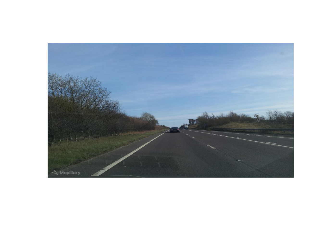
## [1] "Displaying mapillary image close to lon=-4.328339 and lat=55.873593"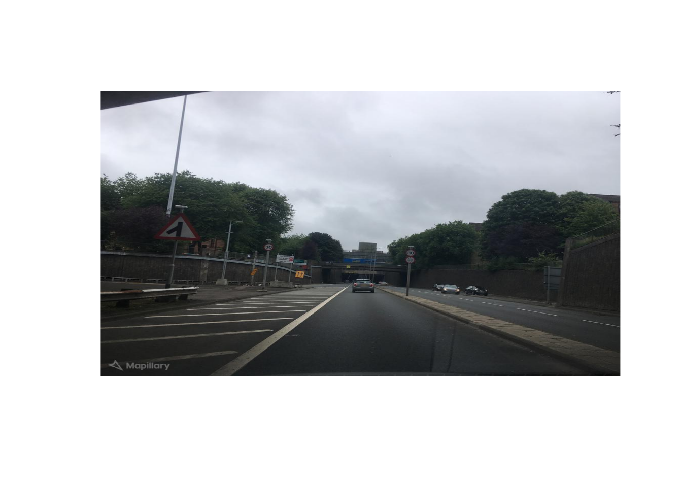
## [1] "Displaying mapillary image close to lon=-0.561374 and lat=51.914048"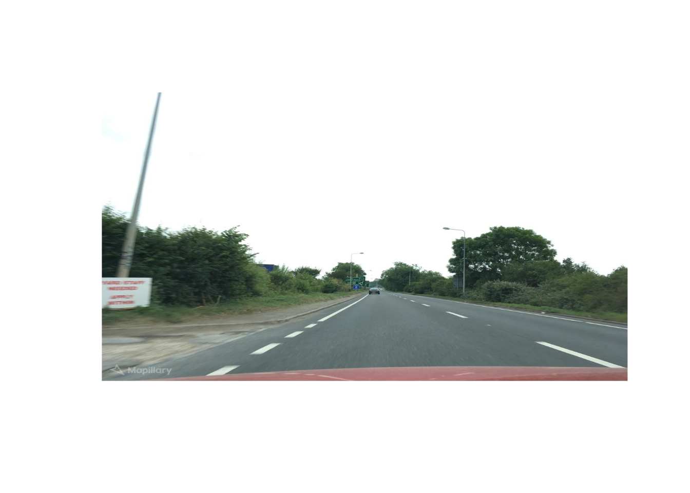
## [1] "Displaying mapillary image close to lon=0.003746 and lat=52.614004"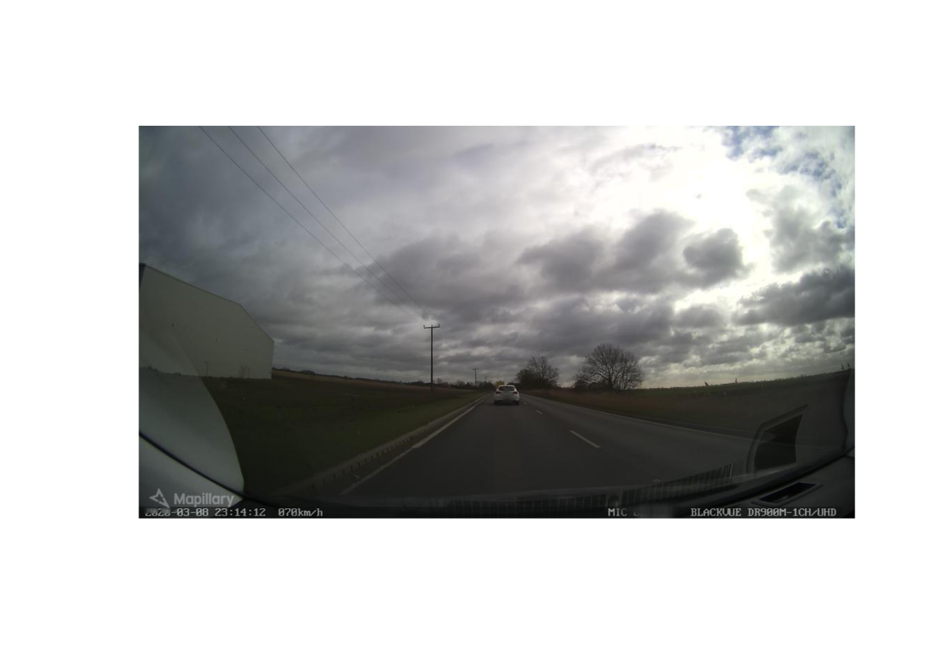
## [1] "Displaying mapillary image close to lon=-1.197392 and lat=51.250871"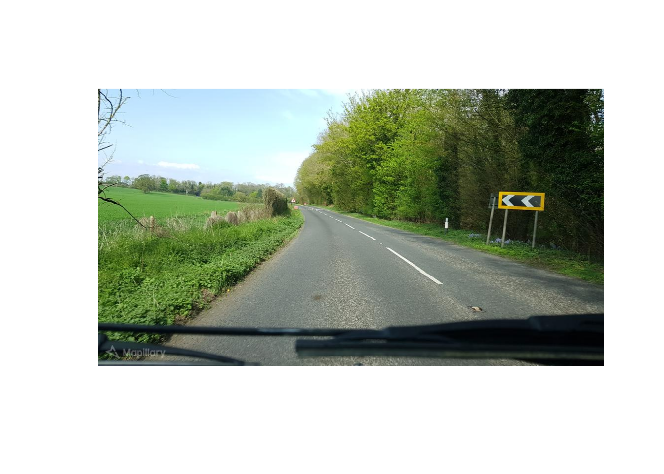
Casualties
Initial exploration
Let’s see how many observations do we have as well as the variables’ number and types.
| Name | casualties2018 |
| Number of rows | 160597 |
| Number of columns | 16 |
| _______________________ | |
| Column type frequency: | |
| factor | 13 |
| numeric | 3 |
| ________________________ | |
| Group variables | None |
Variable type: factor
| skim_variable | n_missing | complete_rate | ordered | n_unique | top_counts |
|---|---|---|---|---|---|
| accident_index | 0 | 1 | FALSE | 122635 | 201: 59, 201: 29, 201: 23, 201: 20 |
| casualty_class | 0 | 1 | FALSE | 3 | Dri: 103371, Pas: 34794, Ped: 22432 |
| sex_of_casualty | 0 | 1 | FALSE | 3 | Mal: 95252, Fem: 65305, Dat: 40 |
| age_band_of_casualty | 0 | 1 | FALSE | 12 | 26 : 33242, 36 : 24225, 46 : 22454, 21 : 18187 |
| casualty_severity | 0 | 1 | FALSE | 3 | Sli: 133302, Ser: 25511, Fat: 1784 |
| pedestrian_location | 0 | 1 | FALSE | 12 | Not: 138163, In : 9153, Cro: 3603, On : 2308 |
| pedestrian_movement | 0 | 1 | FALSE | 10 | Not: 138163, Cro: 7274, Unk: 6205, Cro: 4648 |
| car_passenger | 0 | 1 | FALSE | 4 | Not: 131009, Fro: 18048, Rea: 11057, Dat: 483 |
| bus_or_coach_passenger | 0 | 1 | FALSE | 6 | Not: 157064, Sea: 2218, Sta: 956, Ali: 160 |
| pedestrian_road_maintenance_worker | 0 | 1 | FALSE | 4 | No : 153620, Not: 6852, Yes: 87, Dat: 38 |
| casualty_type | 7 | 1 | FALSE | 21 | Car: 90913, Ped: 22432, Cyc: 17550, Mot: 7221 |
| casualty_home_area_type | 0 | 1 | FALSE | 4 | Urb: 115934, Dat: 16594, Rur: 15534, Sma: 12535 |
| casualty_imd_decile | 0 | 1 | FALSE | 11 | Dat: 27345, Mor: 16684, Mos: 16007, Mor: 15893 |
Variable type: numeric
| skim_variable | n_missing | complete_rate | mean | sd | p0 | p25 | p50 | p75 | p100 | hist |
|---|---|---|---|---|---|---|---|---|---|---|
| vehicle_reference | 0 | 1 | 1.48 | 2.56 | 1 | 1 | 1 | 2 | 999 | ▇▁▁▁▁ |
| casualty_reference | 0 | 1 | 1.40 | 2.70 | 1 | 1 | 1 | 1 | 991 | ▇▁▁▁▁ |
| age_of_casualty | 0 | 1 | 37.06 | 19.66 | -1 | 22 | 34 | 50 | 102 | ▃▇▅▂▁ |
The table above shows that overall we do not have significant missing data in any of the 16 variables as well as some basic statistics of the (few) numerical variables. Now let’s see the mode for every variable.
From the tables above, we can profile the average casualty in 2018 as a male between 26-35 years old, driver of a car that has an accident in urban areas and gets slightly injured after the accident. Let’s further explore the casualties’ demographics.
Casualties’ demographics
At this level of detail, we cannot see notable differences between genders. Both male and female seem to follow the same age distribution, although admittedly, females absolute numbers are notably smaller in all the ages.
Let’s see if both genders follow same distribution according to accident severity.
As can be seen in the plots above, the number of young females involved in fatal and severe accidents are much lesser than those to their male equals.
Future actions and research
This is the end (for now) of this mock report aimed to know about the STATS19 dataset as well as some new coding. There is still lots of data to be explored that, in turn, will lead to research questions, especially if we combine the different datasets together (thankfully they have an accident_index that will make it possible).
We have seen many unanswered questions in this document, and others that have not been directly mentioned, such as the role of women involved in accidents are usually drivers or not.
Another thing I would love to do is to join vehicles and accidents to see if accidents’ severity follows a similar distribution according to the type of vehicles involved. My hypothesis here is that fatal accidents involving cars will be much higher than those involving bicicles, which I expect them to be quite marginal.
Also, I would love to study the impact of the physical conditions of the highways and environment. Although accidents dataset has some information about it, I don’t think it is enough, so, as an OpenStreetMap contributor and advocate, I would love to combine both datasets.
Lovelace, R., Morgan, M., Hama, L., Padgham, M., Ranzolin, D., & Sparks, A. (2019). stats 19: A package for working with open road crash data. The Journal of Open Source Software, 4(33), 1181. https://doi.org/10.21105/joss.01181↩