Mapping and the geospatial ecosystem in R

Warwick-R User Group

Carlos Cámara-Menoyo

June 10, 2024

About me

Carlos Cámara-Menoyo

Senior Research Software Engineer
Centre for Interdisciplinary Methodologies

I love maps and data visualisation.

https://carloscamara.es/en | @ccamara@scholar.social

And R, and participation, and OpenStreetMap, and many other stuff. If you want to know more about me, you can find me here:

“How can I create a map using R?”

That’s the question I’ve been asked a lot, and the question I will try to answer today (kind of)

Aims

• Provide an overview of the mapping process in R
  • Identifying different components of a map
  • Introducing different R packages for specific tasks
• Provide the theoretical foundations to understand the (many) tutorials about maps and geospatial information (with R)
• Provide some basic code examples to highlight basic concepts and packages

Out of scope:

• Not a course on cartography or creating beautiful data visualisations or maps
• Not a course about Spatial operations -> Read https://r.geocompx.org/ by Robin lovelace
• Not an advanced training on any of the packages used

What’s a map?

This is probably the map we are more familiar with: a routing map for cars, usually populated by Google

Points’ map

Map using colour-coded markers with icons

Choropleth Maps

Here we are mapping values (numerical or categorical) to polygon’s background colours

Heatmaps

Heatmaps show density of information

An excellent tutorial by Andrew Heiss on doing a Middle Earth Map ussing {ggplot} and {sf}

• Maps are serious, but can be fun!
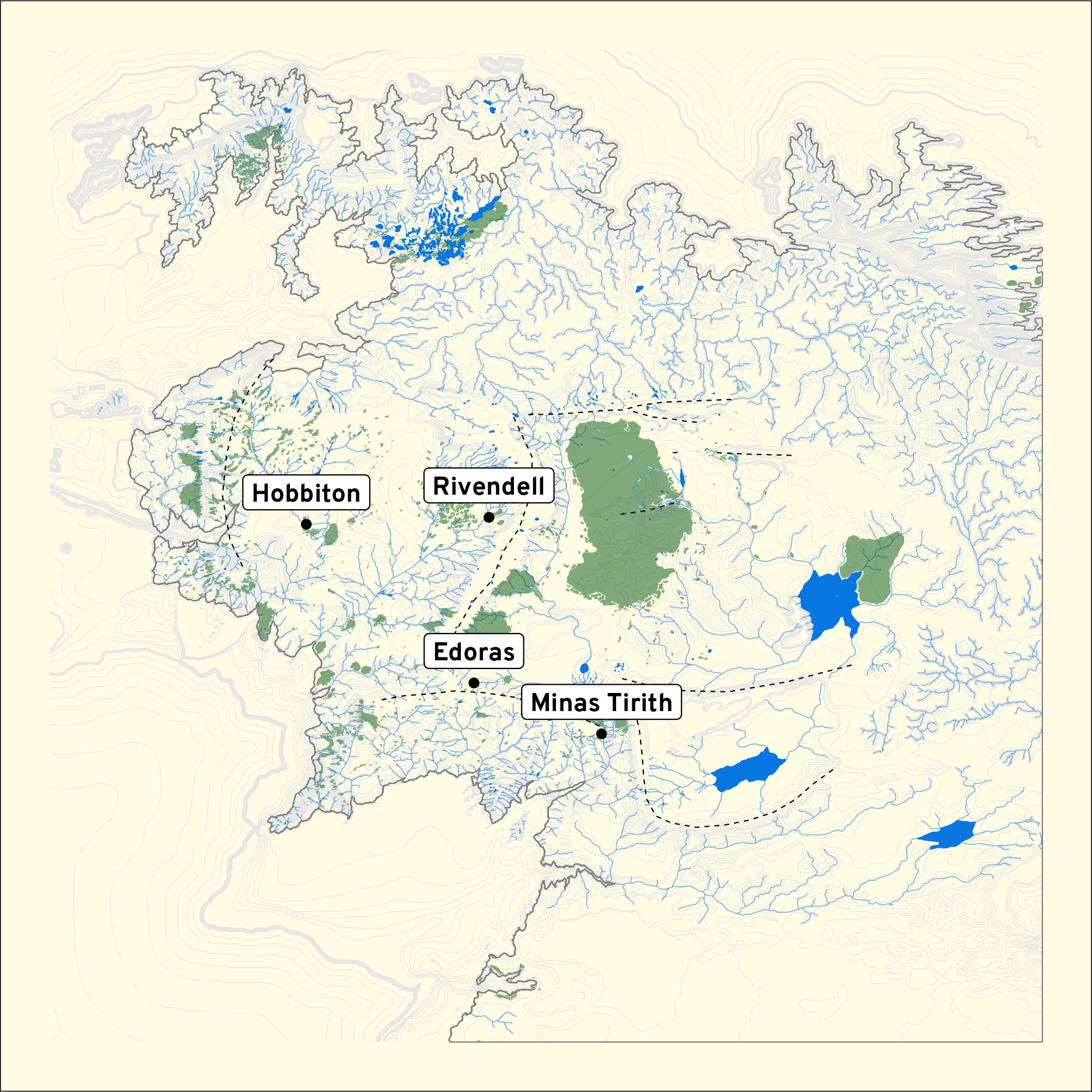
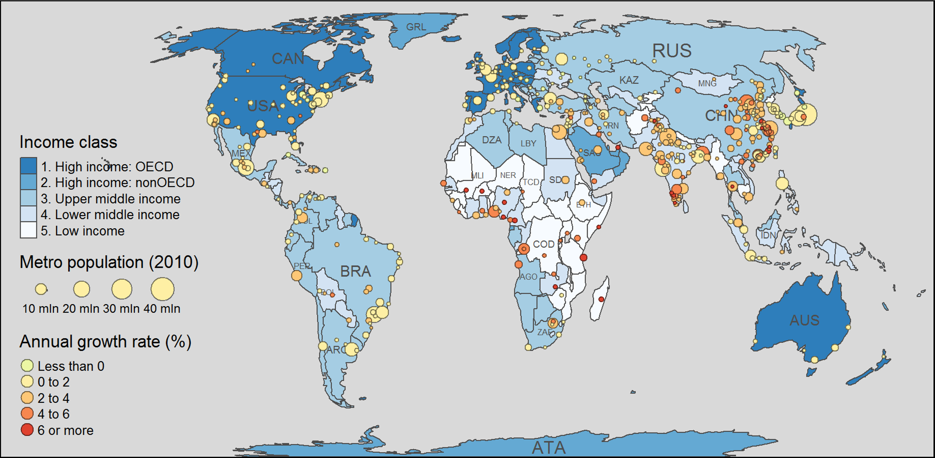
• We can map almost anything (even Pokemons or Middle Earth)

There’s no such thing as “a map”!

• Maps can serve different purposes
• There are many types of maps
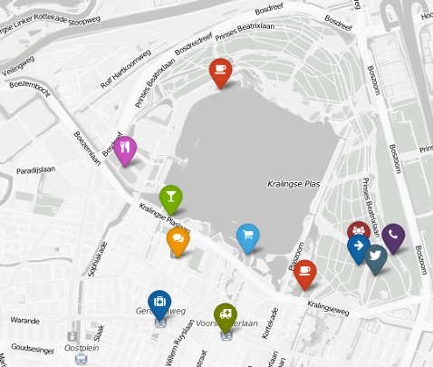
  • Maps are more than routing maps (usually powered by Google)
  • Maps are more than what Google maps or political maps
• Maps can be static (images) or interactive (web, apps)
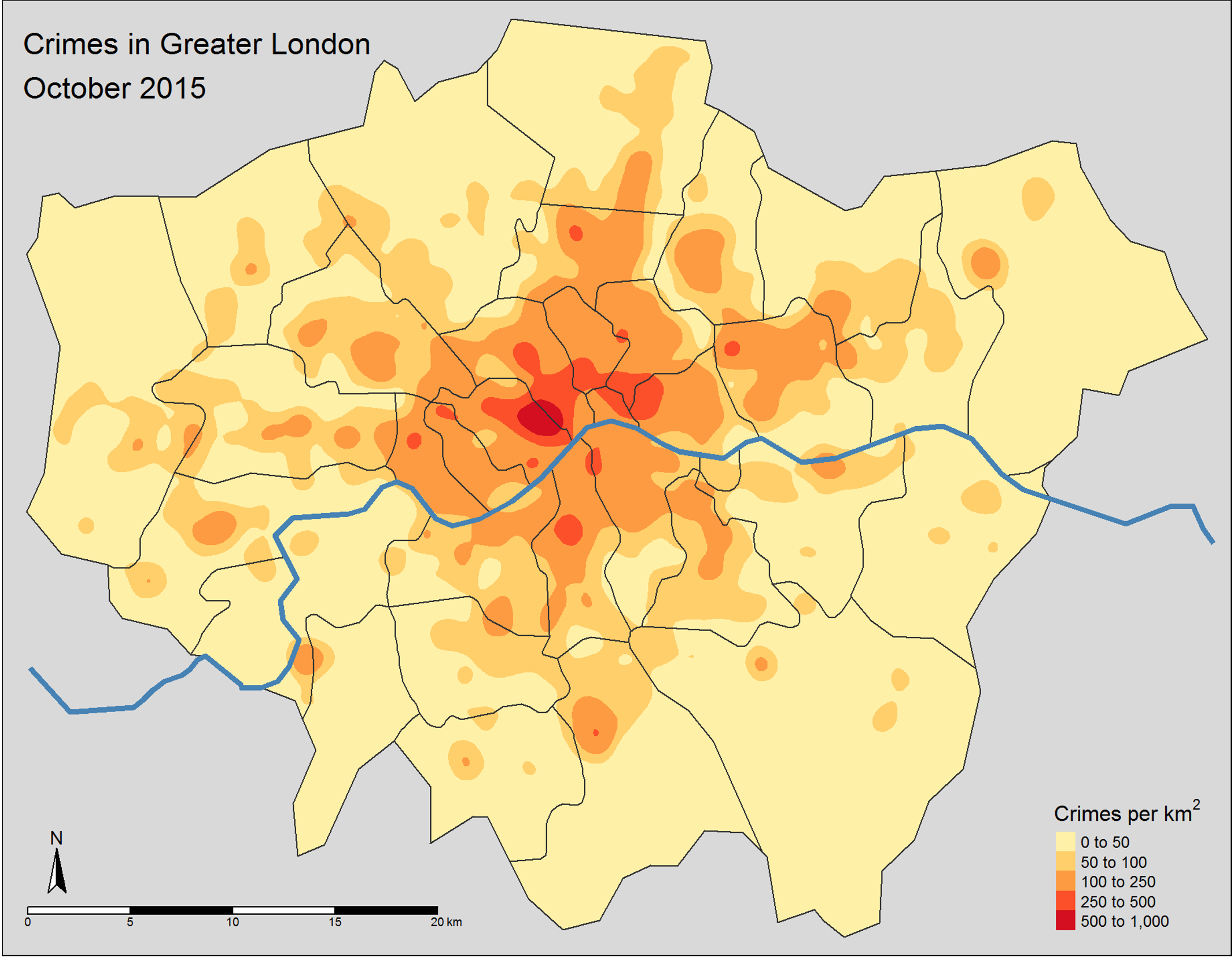
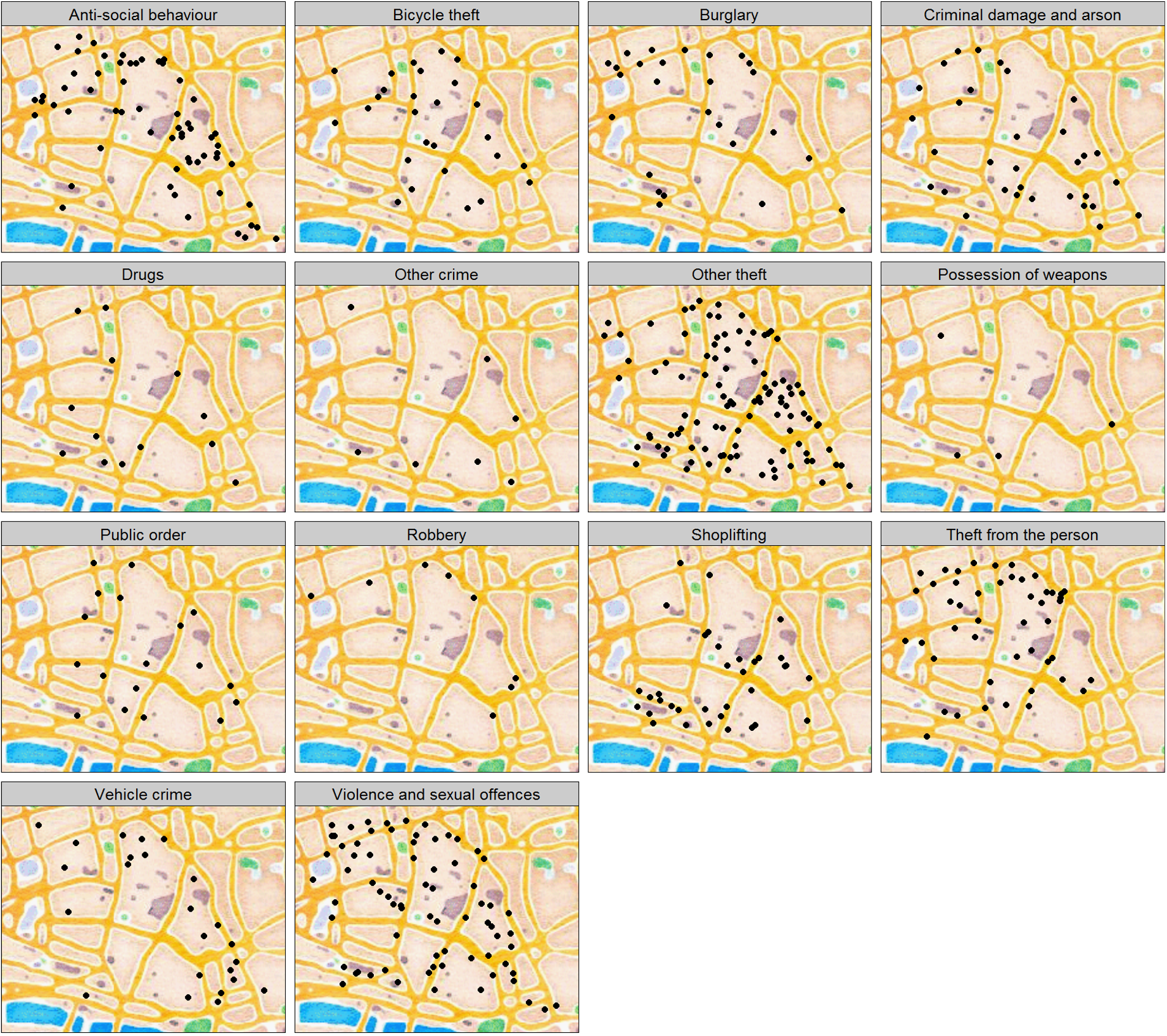
• Maps can visualise information in different ways (points, choropleth, facets…)
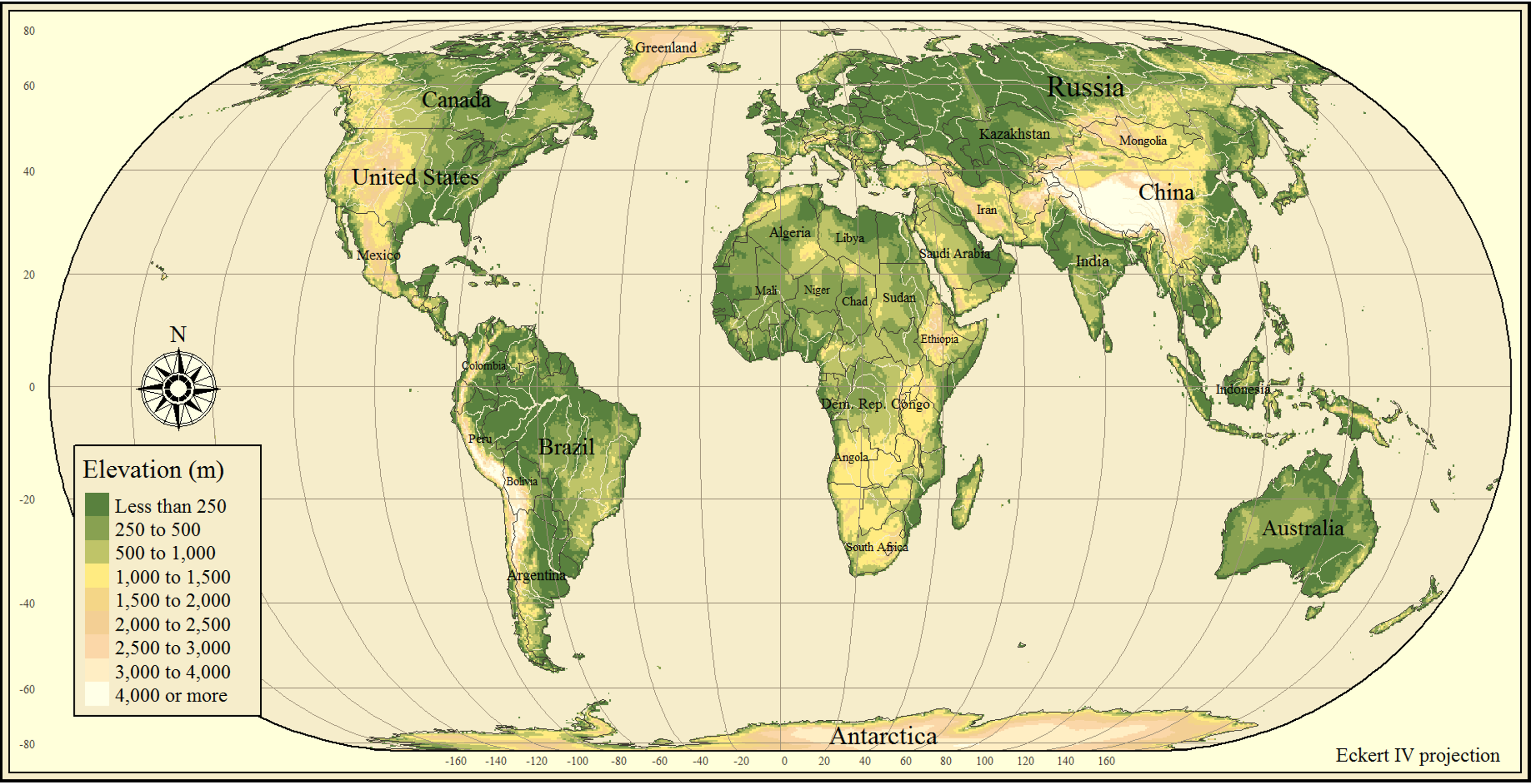
• Maps are subjective (aka political) (i.e. north, center, projections…)

But there’s something they all have in common…

Spatial data

Spatial data: overview

Spatial data situates something in the space (world*). Because of Earth is round and maps are usually flat, spatial data needs to be projected using Coordinate Reference Systems (CRS)

Spatial data is different than regular data (i.e. dataframe) because it contains:

• Geometry: coordinates defining and situating a point, line or polygon

• Attributes for every geometry (variables and values)

• Coordinate Reference System (CRS)

Currently, R’s data structure to stores spatial data is a sf object (or spatial data frame), provided by {sf} - Simple Features for R.

* But it could be something else, like the Moon, Middle Earth…

Types of spatial data

According to how spatial information is stored:

• Vector: geometry is defined by their coordinates
• Raster: made of pixels. Are thematic (i.e. land cover)

According to their geometry (Vectors) :

• Points expressed as pairs of lat, long, or x, y (i.e. markers).
• Lines edges connecting points (i.e. streets)
• Polygons/Multipolygons closed (i.e. countries’ borders)
• (basemaps)

Source of spatial data:

• From a Spatial format file: .geojson, .geopkg, .shp, .topojson, (.csv)

  sf::read_sf("data/CNTR_RG_20M_2020_4326.gpkg")

• From Open Repositories (ONS Geoportal, Eurostat, …)

• Built in in some specialised packages, such as {spData} or {tmap}

• Geocoding: translating addresses to coordinates

• APIs like OpenStreetMap or Eurostat’s GISCO.

• Our own processes and analysis (using R)

R packages by purpose

• Spatial data
  • {sf}: provides data structure for spatial data
  • {sp} (superseeded)
• Geocoding
  • {tidygeocoder}
  • {photon} (unmaintained but working)
• Datasets
  • {spData}: provides spatial datasets (i.e. World country polygons)
  • {giscoR} an API package that helps to retrieve data from Eurostat - GISCO.
  • {osmdata} extract data from OpenStreetMap using Overpass API

• Static visualisation
  • base R plots
  • {ggplot} (+ {ggspatial})
  • {tmap} creates thematic maps using grammar of graphics
  • {mapsf} maps sf objects on base graphics.
• Interactive visualisation
  • {leaflet} (+{leaflet.extras})
  • {tmap}
  • {plotly}
  • {highcharter}

Note that the R ecosystem has changed a lot over time, and older tutorials may talk about deprecated packages such as sp, ggmap, terra…

There are more specialised packages, such as routing, or specific analyses.

Case: Geocoding with {tidygeocoder}

Translating addresses to geographical coordinates

locations <- c("Coventry", "University of Warwick", 
  "Centre for Interdisciplinary Methodologies" )

# Tidycoder needs a data frame structure.
locations_df <- as.data.frame(locations)

library(tidygeocoder)

# geocode the addresses
lat_longs <- locations_df |> 
  geocode(locations, method = 'osm', lat = latitude , long = longitude)

lat_longs

# A tibble: 3 × 3
  locations                                  latitude longitude
  <chr>                                         <dbl>     <dbl>
1 Coventry                                       52.4     -1.51
2 University of Warwick                          52.4     -1.56
3 Centre for Interdisciplinary Methodologies     52.4     -1.56

# Visualise
library(leaflet)

leaflet(lat_longs) |> 
  addTiles() |>
  addMarkers(popup=~locations)

Case: Simple point “map” with base R

Loading the “spatial” data

We will read a csv file containing the latitude and longitude of cities in the world:

cities_world <- read.csv("data/worldcities.csv")

# Check the class
class(cities_world)

[1] "data.frame"

head(cities_world, 3)

     city city_ascii     lat      lng   country iso2 iso3 admin_name capital
1   Tokyo      Tokyo 35.6897 139.6922     Japan   JP  JPN      Tōkyō primary
2 Jakarta    Jakarta -6.1750 106.8275 Indonesia   ID  IDN    Jakarta primary
3   Delhi      Delhi 28.6100  77.2300     India   IN  IND      Delhi   admin
  population         id
1   37732000 1392685764
2   33756000 1360771077
3   32226000 1356872604

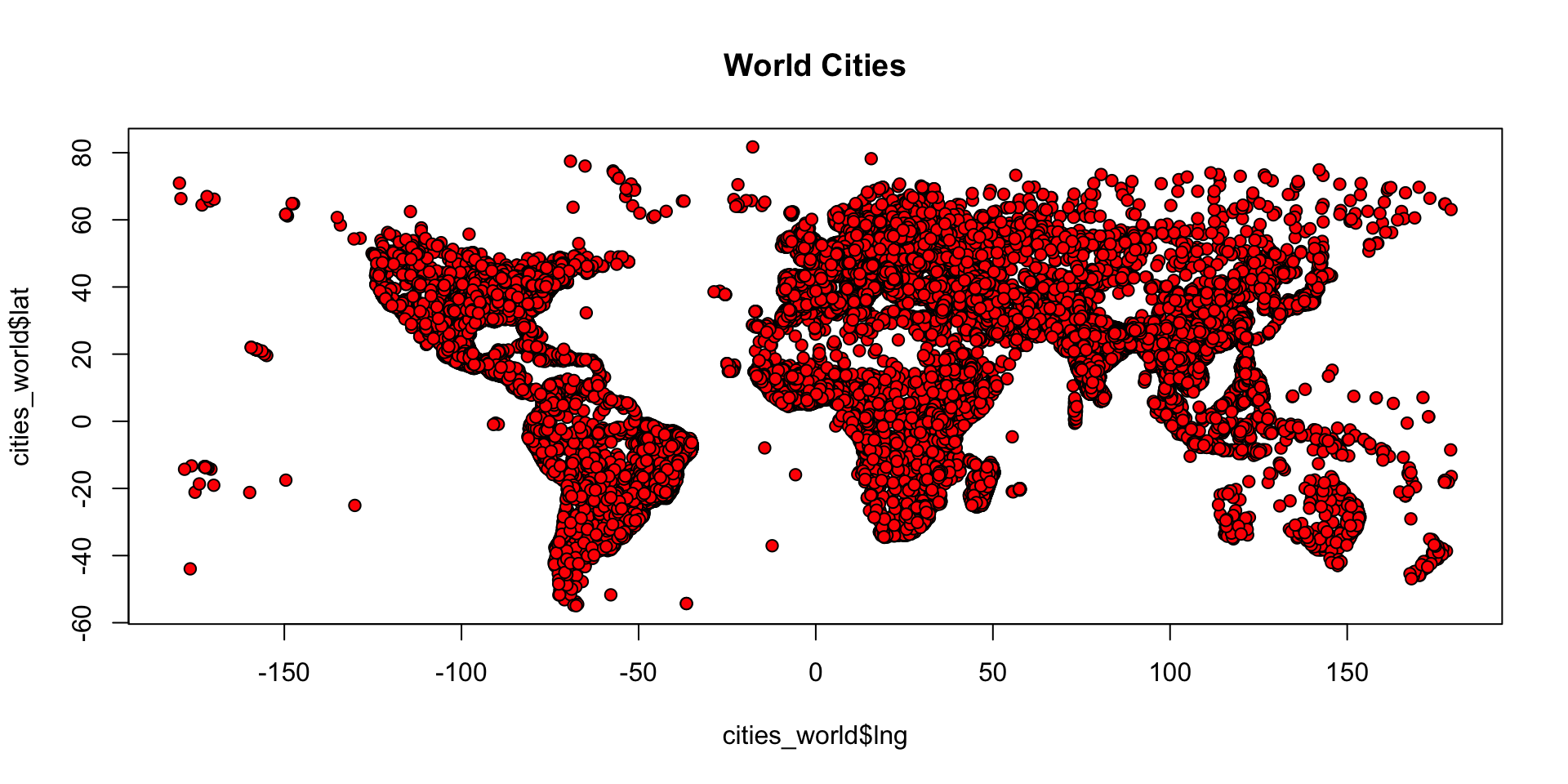
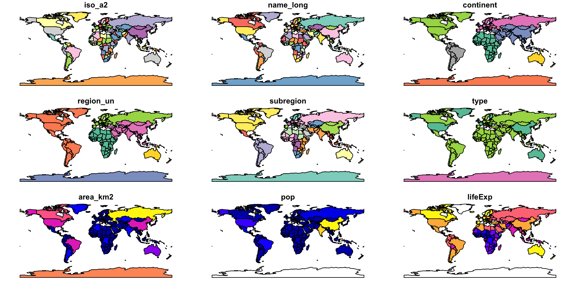
Using base R to visualise the “spatial” data

Latitude and longitude are numbers that can position a point in the world, in a similar way than x and y work in cartesian space. -> We can use base R’s plot():

plot(cities_world$lng, cities_world$lat, 
     pch = 21, bg = "red", main="World Cities")

Is this a good map?

Sure, we could improve this visualisation (i.e. removing borders, axis, map size according to population, adding a background…)

Is this even a map?

Fair point! Is this really a spatial visualisation or a regular visualisation that we read as a geographical space?

We are getting philosophical here!

I sense your frustration. I know what you’re thinking now:

Case: Simple choropleth map of the world with well-known packages

We will use base R and {ggplot} to visualise spatial data creating choropleth maps.

Retrieving data

In this case, we will be be using data provided by the spData package:

library(sf)

# Load built-in data.
world <- spData::world

# Check object's type (pay attention to the output!)
str(world)

sf [177 × 11] (S3: sf/tbl_df/tbl/data.frame)
 $ iso_a2   : chr [1:177] "FJ" "TZ" "EH" "CA" ...
 $ name_long: chr [1:177] "Fiji" "Tanzania" "Western Sahara" "Canada" ...
 $ continent: chr [1:177] "Oceania" "Africa" "Africa" "North America" ...
 $ region_un: chr [1:177] "Oceania" "Africa" "Africa" "Americas" ...
 $ subregion: chr [1:177] "Melanesia" "Eastern Africa" "Northern Africa" "Northern America" ...
 $ type     : chr [1:177] "Sovereign country" "Sovereign country" "Indeterminate" "Sovereign country" ...
 $ area_km2 : num [1:177] 19290 932746 96271 10036043 9510744 ...
 $ pop      : num [1:177] 8.86e+05 5.22e+07 NA 3.55e+07 3.19e+08 ...
 $ lifeExp  : num [1:177] 70 64.2 NA 82 78.8 ...
 $ gdpPercap: num [1:177] 8222 2402 NA 43079 51922 ...
 $ geom     :sfc_MULTIPOLYGON of length 177; first list element: List of 3
  ..$ :List of 1
  .. ..$ : num [1:5, 1:2] -180 -180 -180 -180 -180 ...
  ..$ :List of 1
  .. ..$ : num [1:9, 1:2] 178 178 177 177 178 ...
  ..$ :List of 1
  .. ..$ : num [1:8, 1:2] 180 180 179 179 179 ...
  ..- attr(*, "class")= chr [1:3] "XY" "MULTIPOLYGON" "sfg"
 - attr(*, "sf_column")= chr "geom"
 - attr(*, "agr")= Factor w/ 3 levels "constant","aggregate",..: NA NA NA NA NA NA NA NA NA NA
  ..- attr(*, "names")= chr [1:10] "iso_a2" "name_long" "continent" "region_un" ...

This is a sf object, which is very similar to well-known data frames.

That means that, internally, spData uses sf.

sf objects draw many similarities with data frames, so we can use well-known functions:

# This looks very similar to a dataframe
head(world, 3)

Simple feature collection with 3 features and 10 fields
Geometry type: MULTIPOLYGON
Dimension:     XY
Bounding box:  xmin: -180 ymin: -18.28799 xmax: 180 ymax: 27.65643
Geodetic CRS:  WGS 84
# A tibble: 3 × 11
  iso_a2 name_long  continent region_un subregion type  area_km2     pop lifeExp
  <chr>  <chr>      <chr>     <chr>     <chr>     <chr>    <dbl>   <dbl>   <dbl>
1 FJ     Fiji       Oceania   Oceania   Melanesia Sove…   19290.  8.86e5    70.0
2 TZ     Tanzania   Africa    Africa    Eastern … Sove…  932746.  5.22e7    64.2
3 EH     Western S… Africa    Africa    Northern… Inde…   96271. NA         NA  
# ℹ 2 more variables: gdpPercap <dbl>, geom <MULTIPOLYGON [°]>

Can you spot any difference with regular data frames?

Check speaker’s notes for solution! (press s)

Visualising an sf with base R

Note that plot() reacts slightly differently when passing a sf object:

# Plotting the entire sf object
plot(world)

Plotting a single variable

• Categorical variable
• Numerical variable

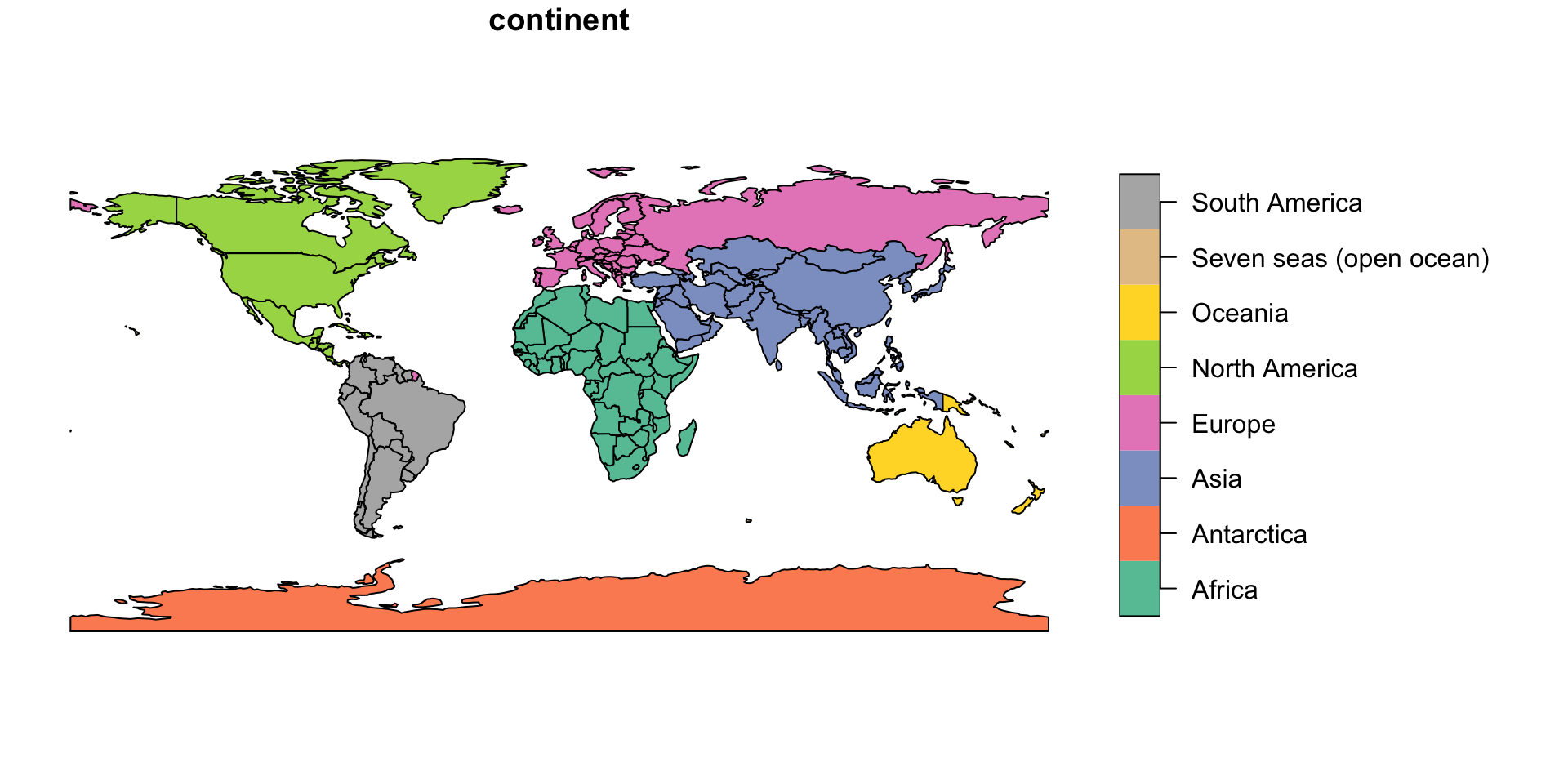
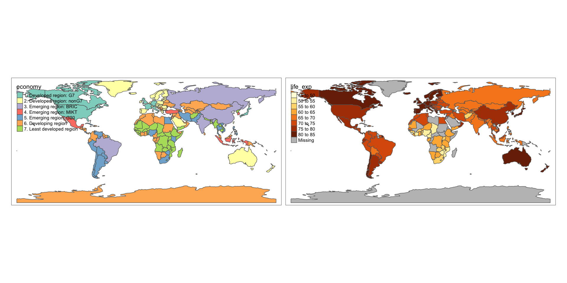
# Plotting a categorical attribute
plot(world["continent"])

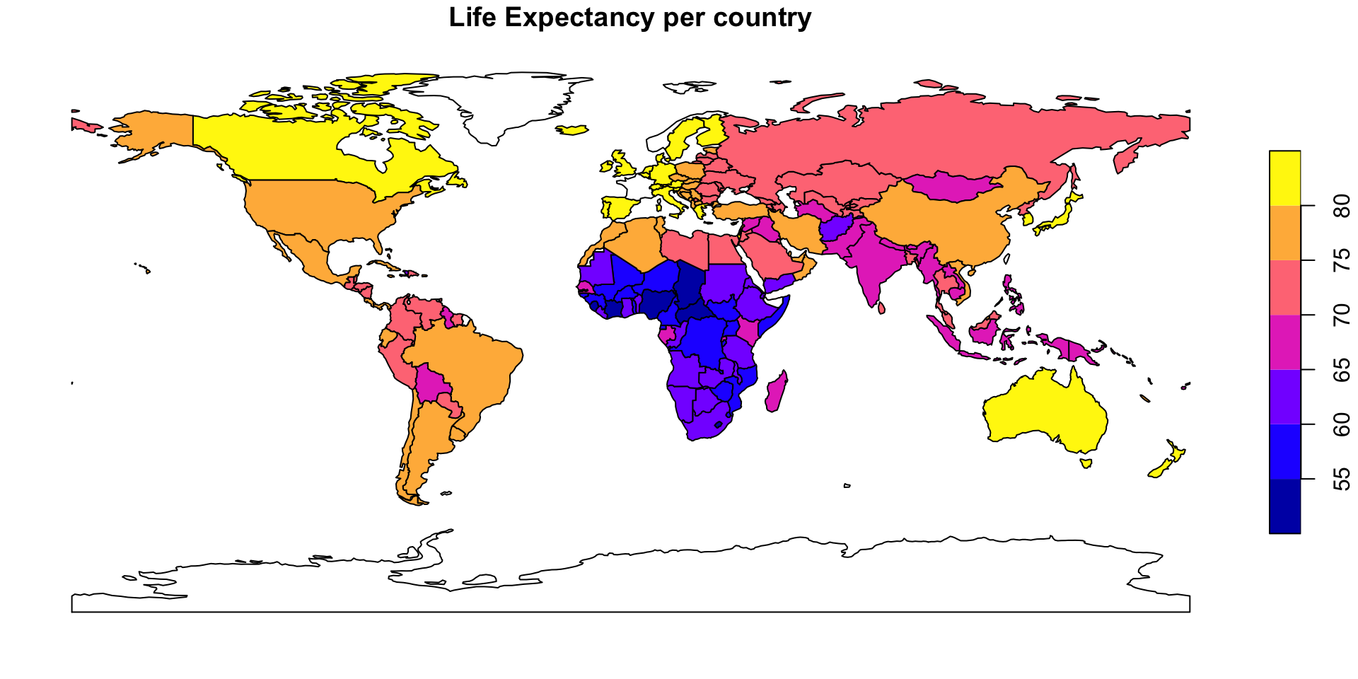
# Plotting a categorical attribute
plot(world["lifeExp"], main = "Life Expectancy per country")

Admittedly, we could use our expertise in data visualisation and base R graphics to dramatically improve this to better communicate our findings, i.e., colour scale, cutters, legend, title…but it’s good enough. And quick!

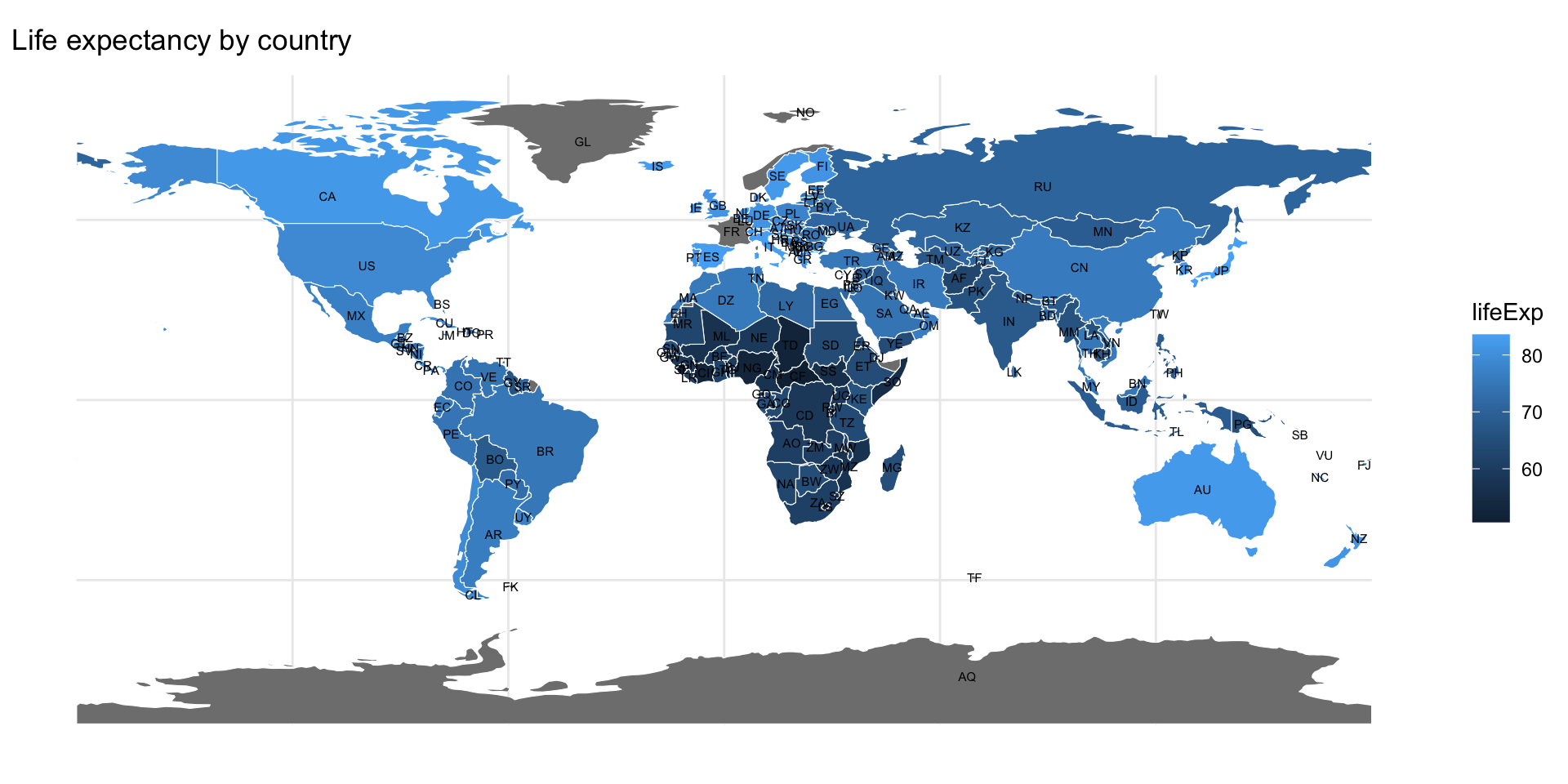
Visualising with {ggplot}

Some may be more familiar with {ggplot}, so we can use it, too (using “new” geom_ functions):

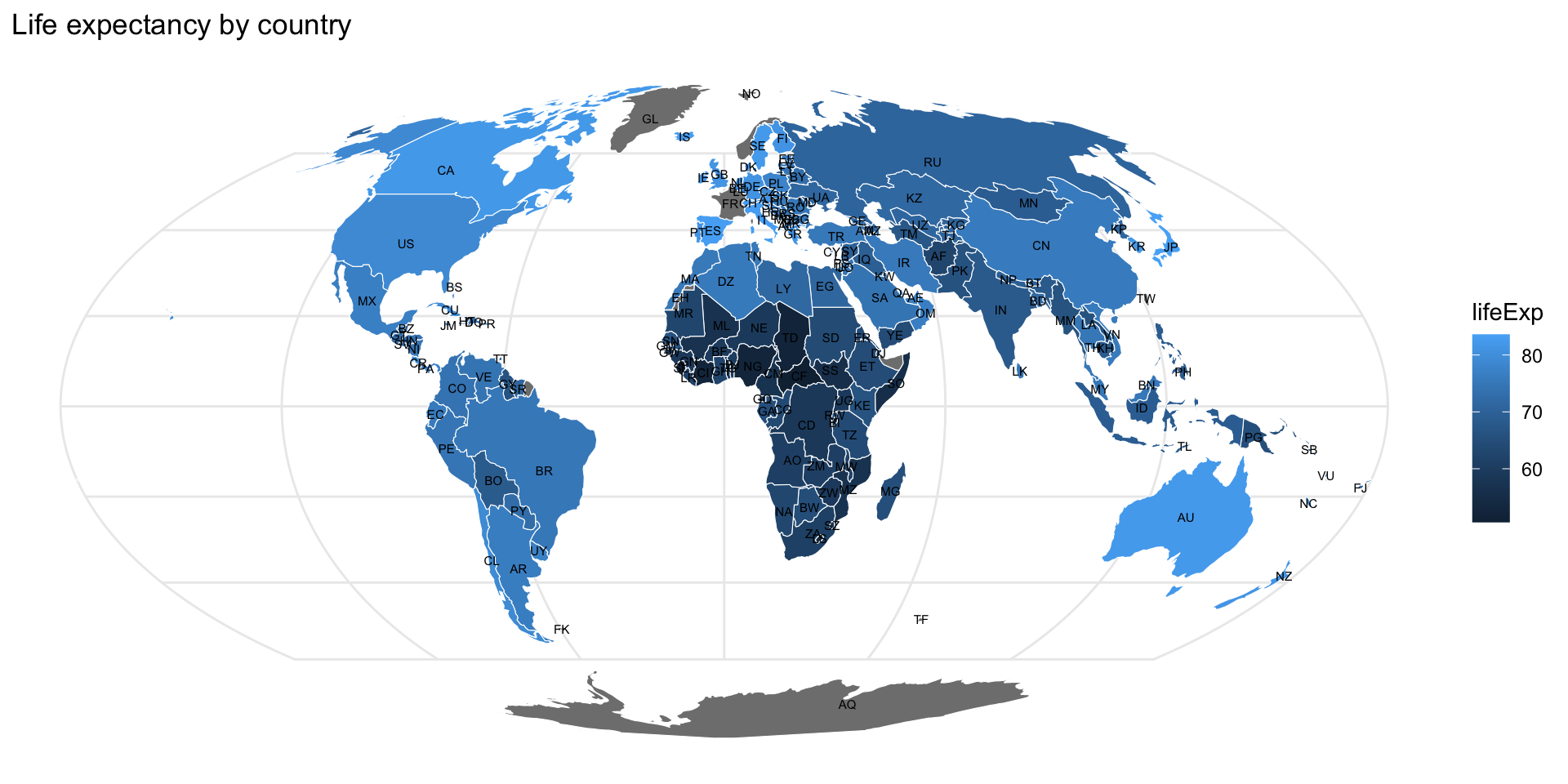
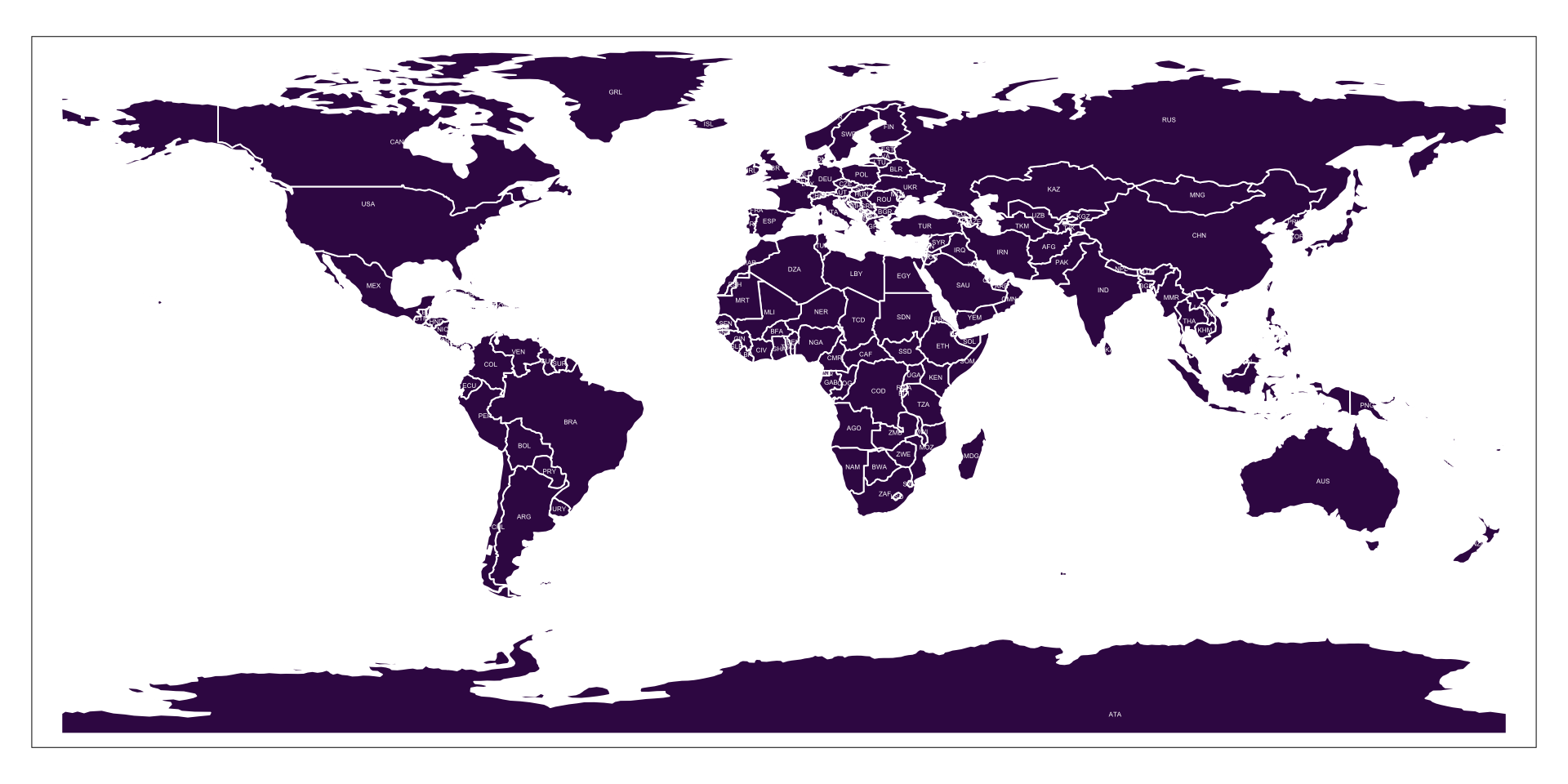
library(ggplot2)

plot_ggchoro <- ggplot(world) +
  # geom_sf is used to visualise sf geometries
  geom_sf(color = "white", aes(fill = lifeExp)) +
  # geom_sf_text visualises the value of a column based on their geometries
  geom_sf_text(aes(label = iso_a2), size = 2) + 
  # Add a title and hide x and y labels.
  labs(title = "Life expectancy by country",
       x = NULL, y = NULL) +
  theme_minimal()

# Result in next slide
plot_ggchoro

But there is more!

Because we are working with an sf, we can visualise it in a different Coordinate Reference System (CRS)

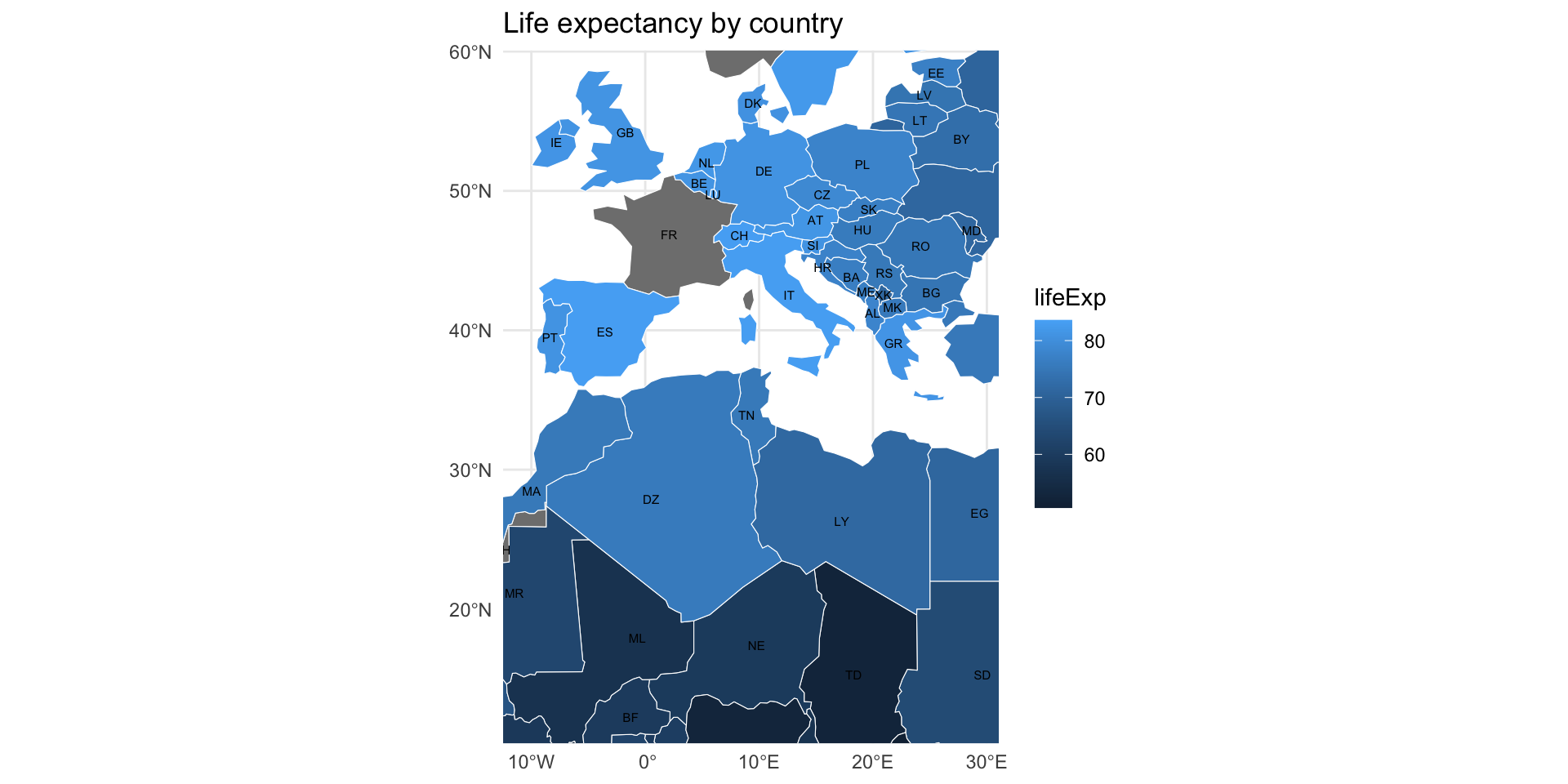
plot_ggchoro + # We are reusing the ggplot from the previous code
  coord_sf(crs = st_crs(3035)) #st_crs is provided by sf

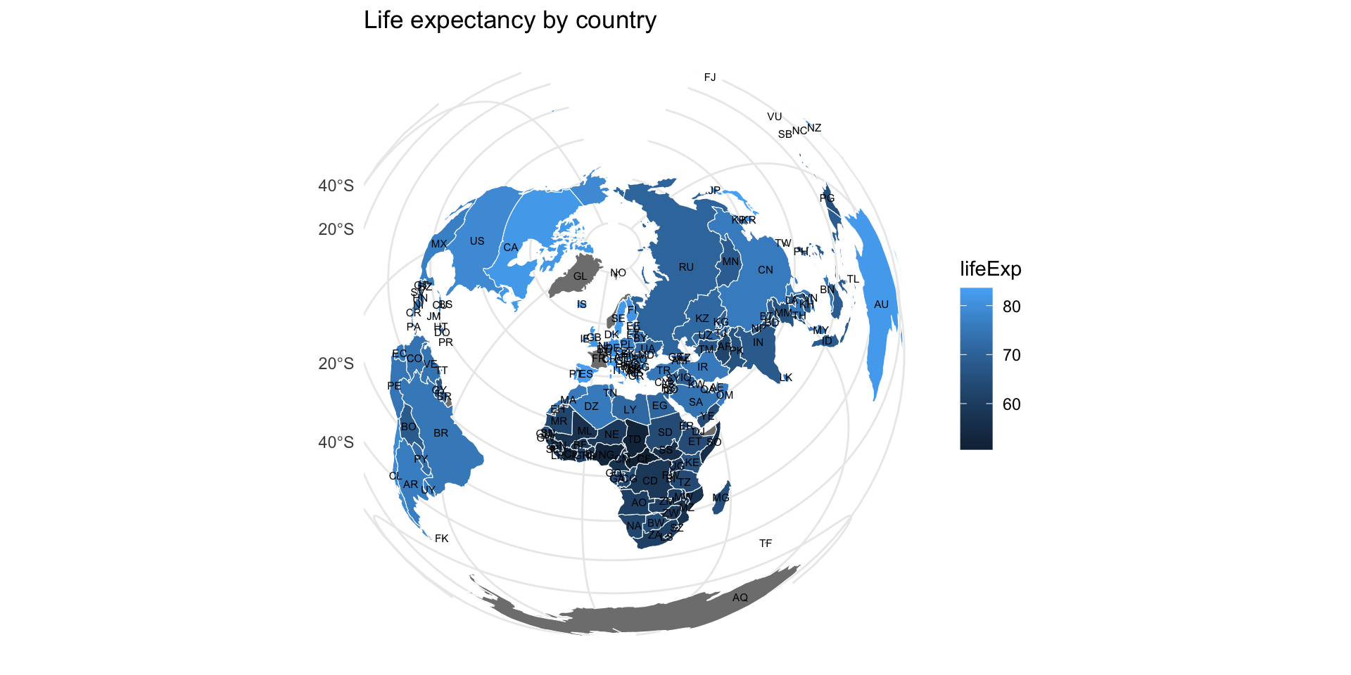
plot_ggchoro + # We are reusing the ggplot from the previous code
  coord_sf(crs = "+proj=moll") #st_crs is provided by sf

More info: Reprojecting geographic data chapter in Geocmputation with R

# Or zooming in!
plot_ggchoro + 
  coord_sf(xlim = c(-12.48, 31.05), ylim = c(10.37, 60.07),
           expand = FALSE)

Pro-tip: Plotly

We can use plotly::ggplotly() to turn a ggplot map into an interactive map:

plotly::ggplotly(plot_ggchoro)

Recap

• In this example we have used the visualisation tools and methods we are familiar with to viusalise spatial data (as opposed to regular data in the previous example).

• But… we have also seen some of the particularities of using spatial data

In the next examples, we will be using specialised packages for visualising geospatial data

Case: Interactive map using {leaflet}

We will create a couple of (basic) interactive maps like the ones you’re used to see in many websites.

Point maps

library(leaflet)

leaflet(data = cities_world[cities_world$capital == "primary", ]) |> 
  addTiles() |>   # Add default OpenStreetMap map tiles
  addCircles(~lng, ~lat, radius = ~population/100, label=~city)

Choropleth maps

leaflet() |> 
  addTiles() |>  # Add default OpenStreetMap map tiles
  addPolygons(data = world)

# Need to define the cuts, bins and color palette beforehand.
bins <- c(0, 20, 40, 60, 80, 100, Inf)
pal <- colorBin("YlOrRd", domain = world$lifeExp, bins = bins)

map_leaflet <- leaflet() |> 
  addTiles() |>  # Add default OpenStreetMap map tiles
  addPolygons(data = world, fillColor = ~pal(lifeExp),
    weight = 2, opacity = 1, color = "white",
    dashArray = "3", fillOpacity = 0.7) 

map_leaflet

map_leaflet |>  
  addPolygons(data = world, 
    fillColor = ~pal(lifeExp),
    weight = 2,
    opacity = 1,
    color = "white",
    dashArray = "3",
    fillOpacity = 0.7,
    highlightOptions = highlightOptions(
      weight = 5,
      color = "#666",
      dashArray = "",
      fillOpacity = 0.7,
      bringToFront = TRUE))

Combining multiple layers, interaction, fullscreen control and mini-map:

library(leaflet.extras)

labels <- sprintf(
  "<strong>%s</strong><br/>%g years",
  world$name_long, round(world$lifeExp,2)
) %>% lapply(htmltools::HTML)


map_leaflet |> 
  setView(0,1,2) |> 
  addPolygons(data = world, 
    fillColor = ~pal(lifeExp),
    weight = 2,
    opacity = 1,
    color = "white",
    dashArray = "3",
    fillOpacity = 0.7,
    highlightOptions = highlightOptions(
      weight = 5,
      color = "#666",
      dashArray = "",
      fillOpacity = 0.7,
      bringToFront = TRUE),
    label = labels,
    labelOptions = labelOptions(
      style = list("font-weight" = "normal", padding = "3px 8px"),
      textsize = "15px",
      direction = "auto")) |> 
  addCircles(data = cities_world[cities_world$capital == "primary", ],
    ~lng, ~lat, radius = ~population/100) |> 
  addMiniMap() |> 
  addFullscreenControl()

More

• Getting started vignette
• Adding legends
• How to create interactive web maps in R using leaflet package (handbook)
• Leaflet extras

Case: Choropleth map with {tmap}

Tmap is a versatile package to create thematic maps using a layered grammar of graphics approach for maps

Loading and exploring geospatial data

library(tmap)

# Tmap provides a built in dataset called `World```
data(World)

class(World)

[1] "sf"         "data.frame"

head(World, 3)

Simple feature collection with 3 features and 15 fields
Geometry type: MULTIPOLYGON
Dimension:     XY
Bounding box:  xmin: 11.6401 ymin: -17.93064 xmax: 75.15803 ymax: 42.68825
Geodetic CRS:  WGS 84
  iso_a3        name  sovereignt continent           area  pop_est pop_est_dens
1    AFG Afghanistan Afghanistan      Asia  652860 [km^2] 28400000     43.50090
2    AGO      Angola      Angola    Africa 1246700 [km^2] 12799293     10.26654
3    ALB     Albania     Albania    Europe   27400 [km^2]  3639453    132.82675
                    economy             income_grp gdp_cap_est life_exp
1 7. Least developed region          5. Low income    784.1549   59.668
2 7. Least developed region 3. Upper middle income   8617.6635       NA
3      6. Developing region 4. Lower middle income   5992.6588   77.347
  well_being footprint inequality      HPI                       geometry
1        3.8      0.79  0.4265574 20.22535 MULTIPOLYGON (((61.21082 35...
2         NA        NA         NA       NA MULTIPOLYGON (((16.32653 -5...
3        5.5      2.21  0.1651337 36.76687 MULTIPOLYGON (((20.59025 41...

Visualising with {tmap}

Tmap uses a “grammar of graphics” which is very similar to ggplot’s:

tm_shape(World) + 
  tm_borders()

tm_shape(World) + 
  tm_borders(lw = 2, lt=4, col = "blue")

tm_shape(World) +
  tm_fill()

tm_shape(World) +
  tm_fill("well_being")

And we can combine them together!

tm_shape(World) + 
  tm_fill(col = "#3C1053") + 
  tm_borders(col = "white") + 
  tm_text("iso_a3", size = 0.25)

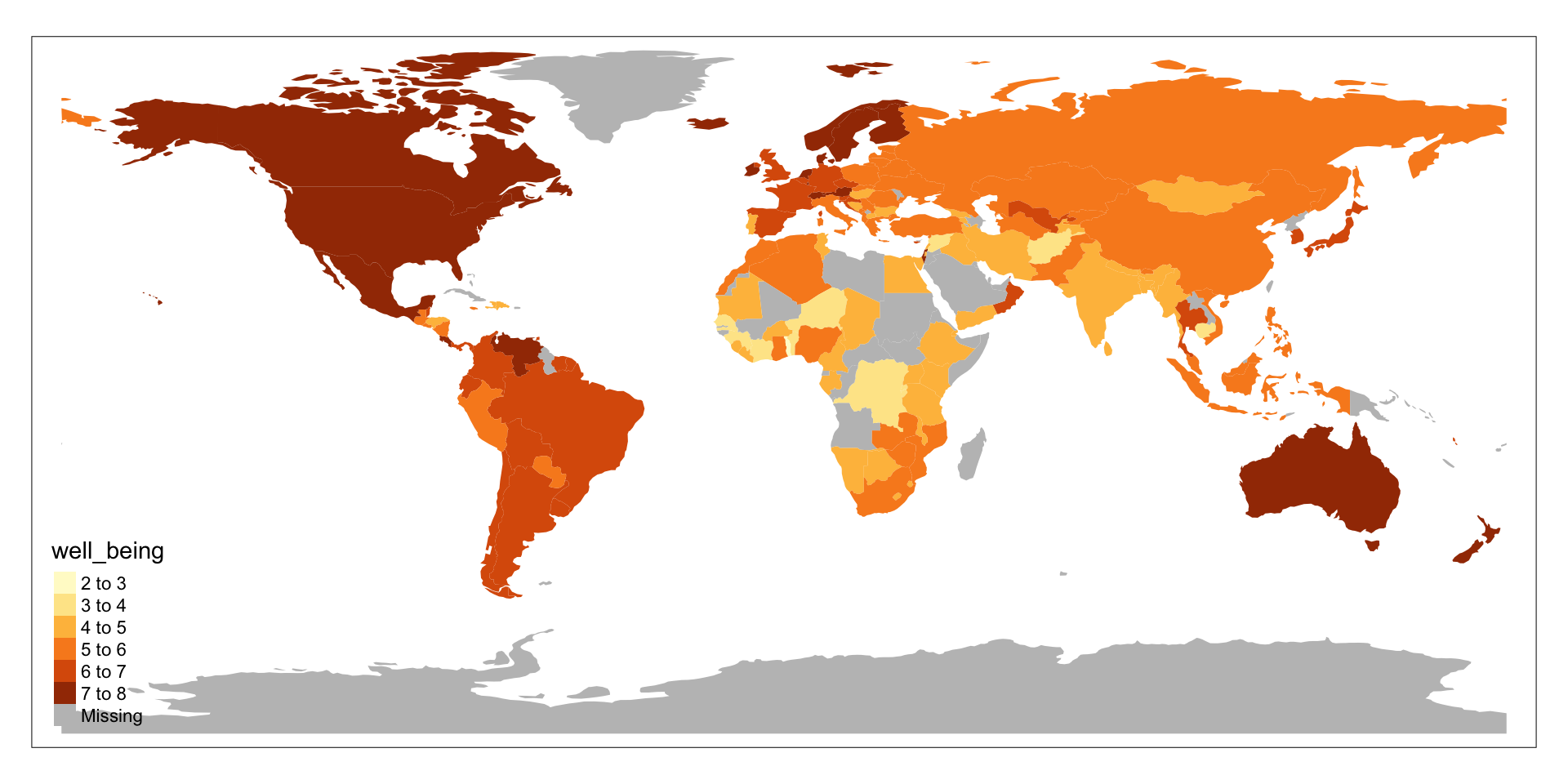
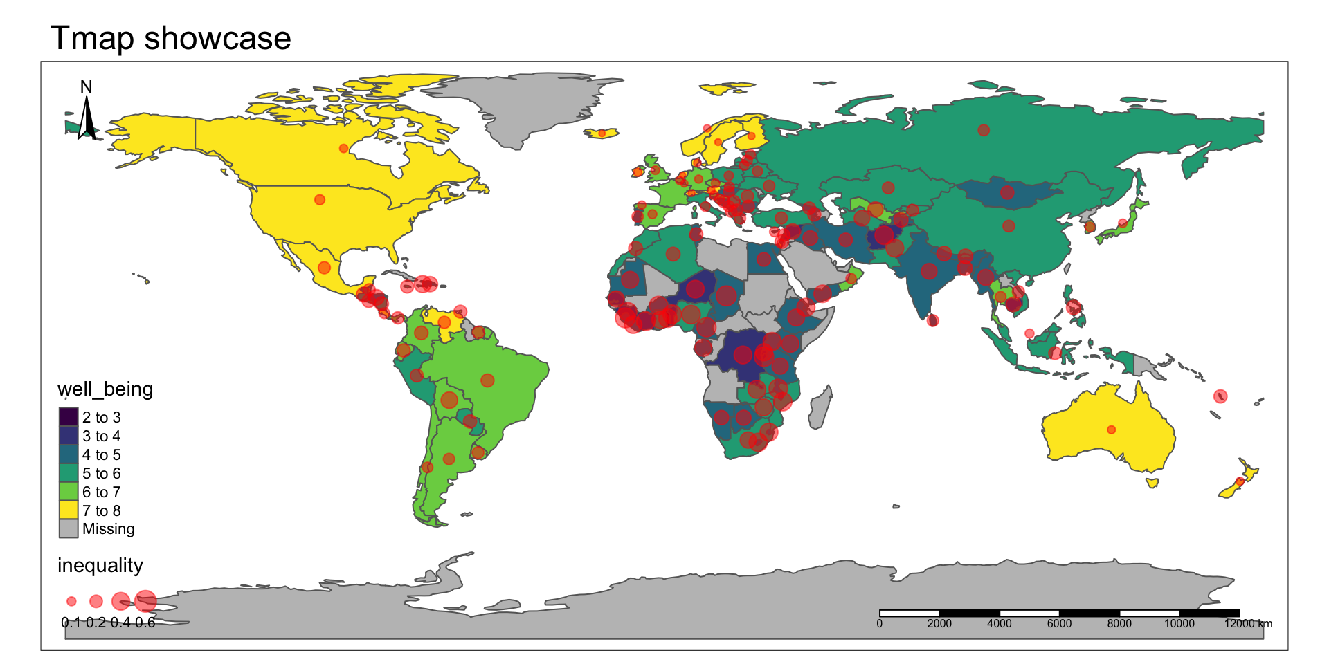
map_demo <- tm_shape(World) +
  tm_polygons("well_being", legend.title = "Happy Planet Index", palette = "viridis") +
  tm_dots(size = "inequality", alpha = 0.5, col = "red") +
  tm_scale_bar() + #Tmap tries to position scale and compass in an empty area, but we can control their position
  tm_compass(position = c("left", "top")) +
  tm_layout(main.title = "Tmap showcase")

map_demo

+info: https://r-tmap.github.io/tmap-book/visual-variables.html

Interactive mapping

tmap_mode("view")

map_demo

Facetting

tmap_mode("plot") # Switch to printed map mode.

map_facet <- tm_shape(World) +
  tm_polygons(c("economy", "life_exp")) +
  tm_facets(ncol = 2,sync = TRUE,)

map_facet

tmap_mode("view")

map_facet

Heatmaps

Heatmaps

Facets / small multiples

Facetted maps

Composite maps

Combining different layers

Theming

Themes

More info about tmap

• Getting started vignette
• Official Tmap handbook
• Geocomputation with R chapter

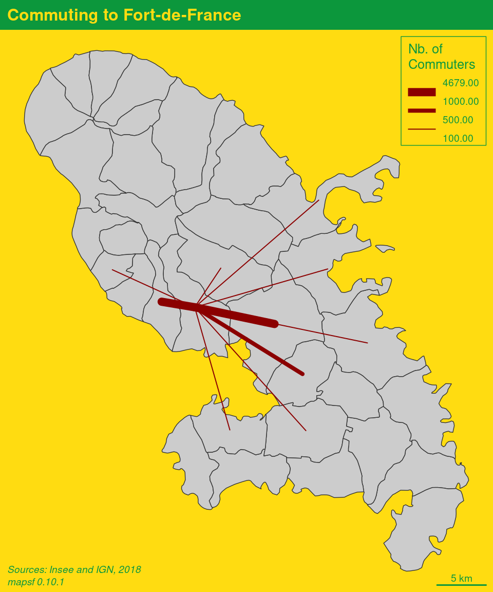
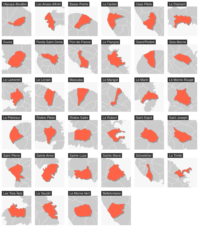
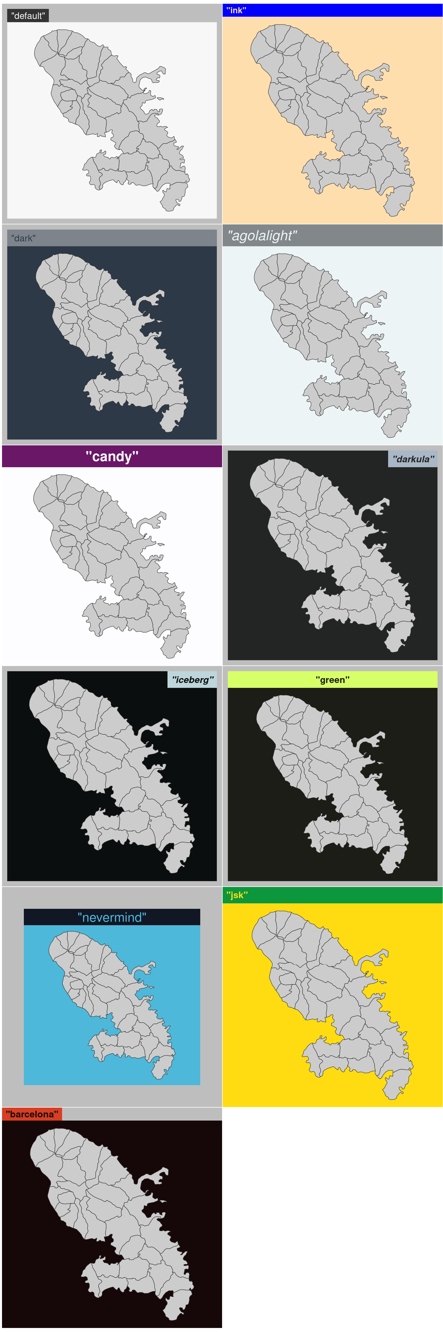
Case: Basic spatial manipulation and visualisation with {mapsf}

Overview

We are going to create a slightly more complex choropleth.

We will be joining two datasets (an sf and a data frame) and overlaying another layer with points.

To do so, we will be using a specialised library: {mapsf}.

Loading data

• englandHealthStats.csv: A regular dataframe with National Statistics Health Index for the Upper Tier Local Authority and Regions over the 2015-2018 (no geometry)

# Read the csv 
englandHealthStats <- read.csv("data/England_all_geog_aggregated_2018.csv")

head(englandHealthStats, 4)

  Area_code            Area_name   ow_obs hyp_ten   low_bw     alc smoke
1 E06000001           Hartlepool 70.44500   17.08 4.648649 1020.75  18.6
2 E06000002        Middlesbrough 64.92679   13.33 3.482881  964.21  17.4
3 E06000003 Redcar and Cleveland 72.50698   17.00 3.249391  806.47  13.5
4 E06000004     Stockton-on-Tees 68.00095   15.08 3.868270  940.14  16.4
  activity   eating sti_screen teen_preg in_eet pupil_abs   ey_dev training
1 59.06190 50.62030   573.3454  38.02535    2.8  14.80276 69.38776     13.4
2 57.93348 53.46347   632.6721  39.35599    4.1  15.51724 63.86139     12.3
3 64.31142 51.93798   500.5548  34.56553    4.3  13.53662 71.44615     17.9
4 61.86028 49.89948   486.5672  26.75159    4.2  12.04075 70.46737     16.8
  ks4_dev low_pay pov_child unempl wp_safety incare_child avoid_mort suicide
1    60.3    34.2      21.4    9.0       270       138.65      312.8    11.6
2    59.2    26.8      30.0    7.4       197       137.36      379.7    15.6
3    61.1    29.1      18.7    5.3       450       103.20      288.0    10.8
4    66.8    24.7      16.8    5.7       341       108.21      275.7     9.2
  inf_mort dementia disability diff_adls kidney frailty cancer diab srwb_sat
1 3.561023     0.94       24.7     43.18   4.91  614.05   3.09 7.08     7.56
2 4.199475     0.79       24.1     38.08   3.37  771.68   2.33 7.30     7.61
3 3.305785     0.97       26.5     38.54   3.47  592.90   3.53 8.19     7.71
4 3.509307     0.99       25.2     38.72   3.91  598.62   2.93 6.92     7.68
  srwb_worth srwb_hap srwb_anx depres semh_child self_harm air_poll
1       7.84     7.39     2.74  11.84      14.99    264.17   7.3237
2       7.92     7.43     2.75   9.76      17.73    391.33   8.0331
3       7.85     7.59     2.61  13.24      17.51    286.55   7.3890
4       7.82     7.60     2.39  14.71      15.30    280.98   7.6095
  pub_greenspace priv_greenspace env_noise road_safety  road_traff rough_sleep
1       637.0132            94.1  5.137170      180.57 0.004616966   3.2174342
2       721.2491            94.6  6.458387      266.14 0.015339576   7.8266747
3       743.7697            94.7  5.376029      198.50 0.002592768   0.7314326
4       799.7353            94.4 13.480146      187.18 0.004795996   1.5211979
  house_afford GP_dist pharm_dist sport_dist crime_pers      hle musculo  resp
1         3.98    0.86       0.86       0.40  113.70412 57.69059   0.735 5.100
2         4.44    0.63       0.63       0.47  141.64147 58.15417   0.750 4.430
3         5.00    0.71       0.71       0.48   83.93189 60.44574   0.620 5.130
4         5.29    0.76       0.76       0.47   90.48085 58.51303   0.740 4.685
    cvd ow_obs_child drug can_screen      vac
1 2.118     34.81375  106   68.73761 89.51405
2 1.814     33.48931  121   66.32224 87.09477
3 2.250     32.51136   91   72.43323 91.39257
4 2.014     30.28729   92   71.14734 93.16532

• boundaries_counties_ua_buc.gpkg: Counties and Unitary Authorities (December 2019) Boundaries UK BUC, from the ONS Geoportal

# Source: 
boundaries_counties_ua_buc <- read_sf("data/CTYUA_Dec_2019_UGCB_in_the_UK_2022_4135466293491974949.gpkg") #20m

head(boundaries_counties_ua_buc, 4)

Simple feature collection with 4 features and 8 fields
Geometry type: MULTIPOLYGON
Dimension:     XY
Bounding box:  xmin: 435563.2 ymin: 507839.1 xmax: 478074.1 ymax: 537152
Projected CRS: OSGB36 / British National Grid
# A tibble: 4 × 9
  ctyua19cd ctyua19nm            ctyua19nmw  bng_e  bng_n  long   lat GlobalID  
  <chr>     <chr>                <chr>       <int>  <int> <dbl> <dbl> <chr>     
1 E06000001 Hartlepool           " "        447160 531474 -1.27  54.7 {70A72826…
2 E06000002 Middlesbrough        " "        451141 516887 -1.21  54.5 {77377060…
3 E06000003 Redcar and Cleveland " "        464361 519597 -1.01  54.6 {922557F5…
4 E06000004 Stockton-on-Tees     " "        444940 518183 -1.31  54.6 {148A3F71…
# ℹ 1 more variable: SHAPE <MULTIPOLYGON [m]>

Combining data together

sf objects are “Spatial Dataframes”, and as such, we can use same operations as those used with regular dataframes, such as dplyr’s joins:

sdf <- dplyr::left_join(boundaries_counties_ua_buc, englandHealthStats, 
                        by = c("ctyua19nm" = "Area_name"))

head(sdf, 4)

Simple feature collection with 4 features and 65 fields
Geometry type: MULTIPOLYGON
Dimension:     XY
Bounding box:  xmin: 435563.2 ymin: 507839.1 xmax: 478074.1 ymax: 537152
Projected CRS: OSGB36 / British National Grid
# A tibble: 4 × 66
  ctyua19cd ctyua19nm            ctyua19nmw  bng_e  bng_n  long   lat GlobalID  
  <chr>     <chr>                <chr>       <int>  <int> <dbl> <dbl> <chr>     
1 E06000001 Hartlepool           " "        447160 531474 -1.27  54.7 {70A72826…
2 E06000002 Middlesbrough        " "        451141 516887 -1.21  54.5 {77377060…
3 E06000003 Redcar and Cleveland " "        464361 519597 -1.01  54.6 {922557F5…
4 E06000004 Stockton-on-Tees     " "        444940 518183 -1.31  54.6 {148A3F71…
# ℹ 58 more variables: SHAPE <MULTIPOLYGON [m]>, Area_code <chr>, ow_obs <dbl>,
#   hyp_ten <dbl>, low_bw <dbl>, alc <dbl>, smoke <dbl>, activity <dbl>,
#   eating <dbl>, sti_screen <dbl>, teen_preg <dbl>, in_eet <dbl>,
#   pupil_abs <dbl>, ey_dev <dbl>, training <dbl>, ks4_dev <dbl>,
#   low_pay <dbl>, pov_child <dbl>, unempl <dbl>, wp_safety <int>,
#   incare_child <dbl>, avoid_mort <dbl>, suicide <dbl>, inf_mort <dbl>,
#   dementia <dbl>, disability <dbl>, diff_adls <dbl>, kidney <dbl>, …

A basic choropleth with {mapsf}

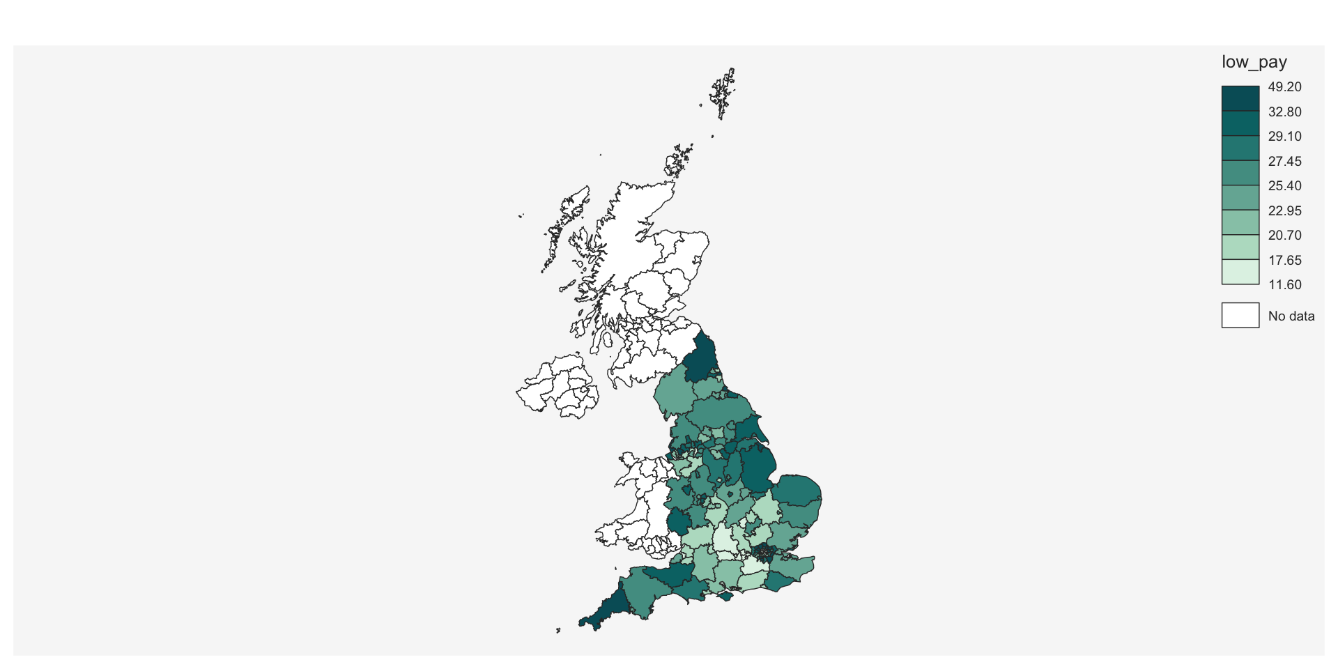
library(mapsf)

mf_map(x = sdf, type = "choro", var = "low_pay")

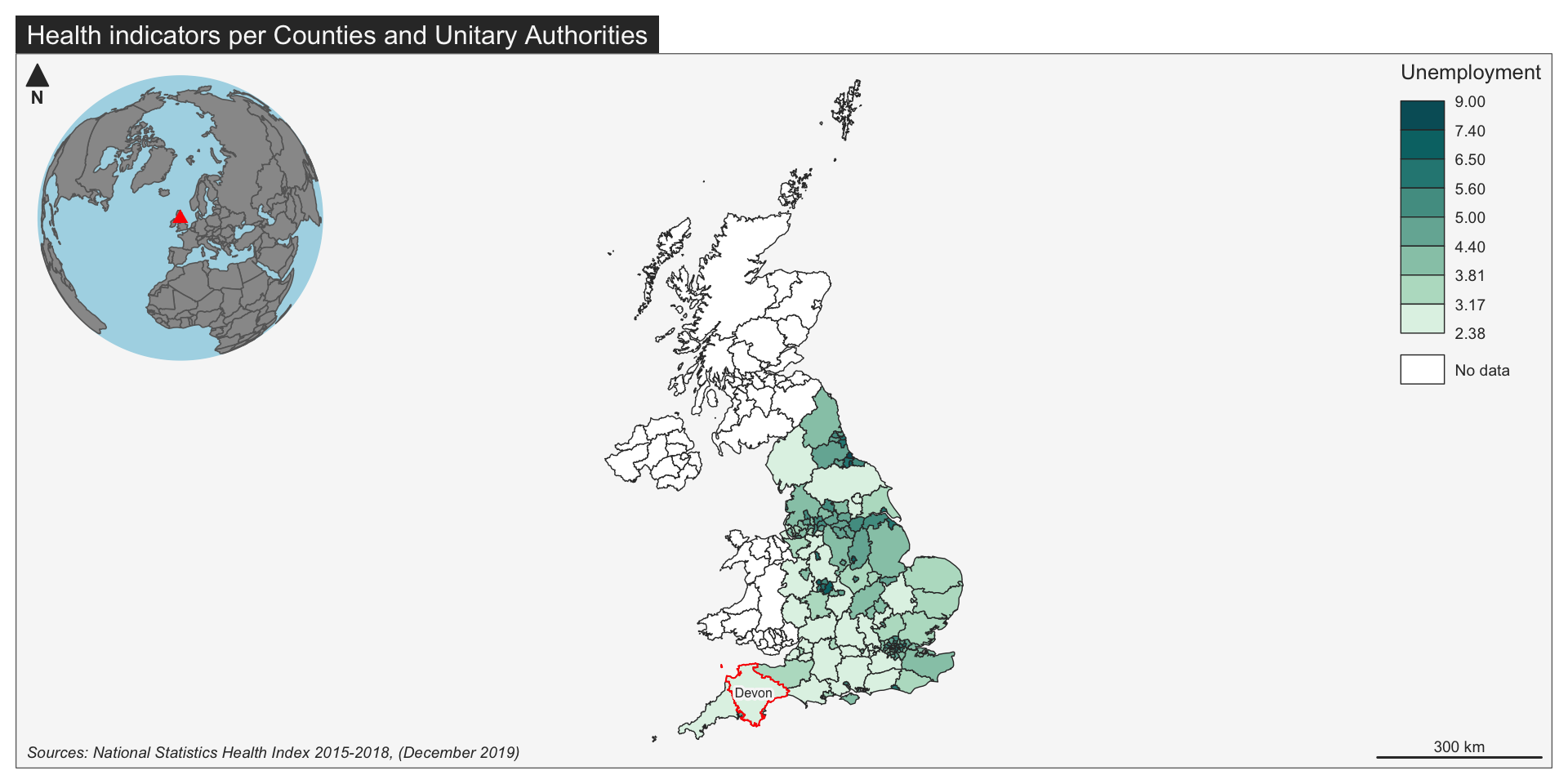
We can improve it further. {mapsf} follows the same logic (And parameters) as base R graphics:

mf_map(x = sdf, type = "choro", var = "unempl",
  leg_title="Unemployment", breaks = "jenks")

# Highlight region with top value
mf_map(x = head(sdf[order(sdf$unempl), ],1), var = "ctyua19nm",
  type = "base", border = "red", lwd = 1, col = NULL, alpha = 0, add = TRUE )

# Labels for the top value
mf_label(
  x = head(sdf[order(sdf$unempl), ],1), var = "ctyua19nm",
  cex = 0.5, halo = TRUE, r = 0.15
)

# Inset map
mf_inset_on(x = "worldmap", pos = "topleft")
mf_worldmap(sdf)
mf_inset_off()

# Layout (title, scale, north and credits)
mf_layout(
  title = "Health indicators per Counties and Unitary Authorities",
  credits = "Sources: National Statistics Health Index 2015-2018, (December 2019)",
  frame = TRUE
)

More…

8 types of maps (+info)

Proportional symbols

Poportional symbols choropleth

Links maps

mapsf can do facetted maps (small multiples)

Facetted maps in a loop

Theming

11 Built-in themes

More info

• Extensive official documentation https://riatelab.github.io/mapsf/
• Tutorial about plotting with base R https://towardsdatascience.com/base-plotting-in-r-eb365da06b22

Wrap up

1. We have a better understanding about what geospatial data and maps are (and what they entail!)
2. We have been introduced to a number of packages, each one performing different functions
3. We have been exposed to code showing affordances and potentialities of packages, to inform our decisions

More…

Of course, there’s way more to know about working with geospatial data in R. If you’re interested, please refer to Geocomputation with R, by Robin Lovelace, Jakub Nowosad and Jannes Muenchow.

…or wait to hear Robin sharing that in an upcoming WRUG session (stay tunned!)

Questions?

Carlos.camara@warwick.ac.uk